
Self-balancing Motorcycle
6. Self-balancing motorcycle
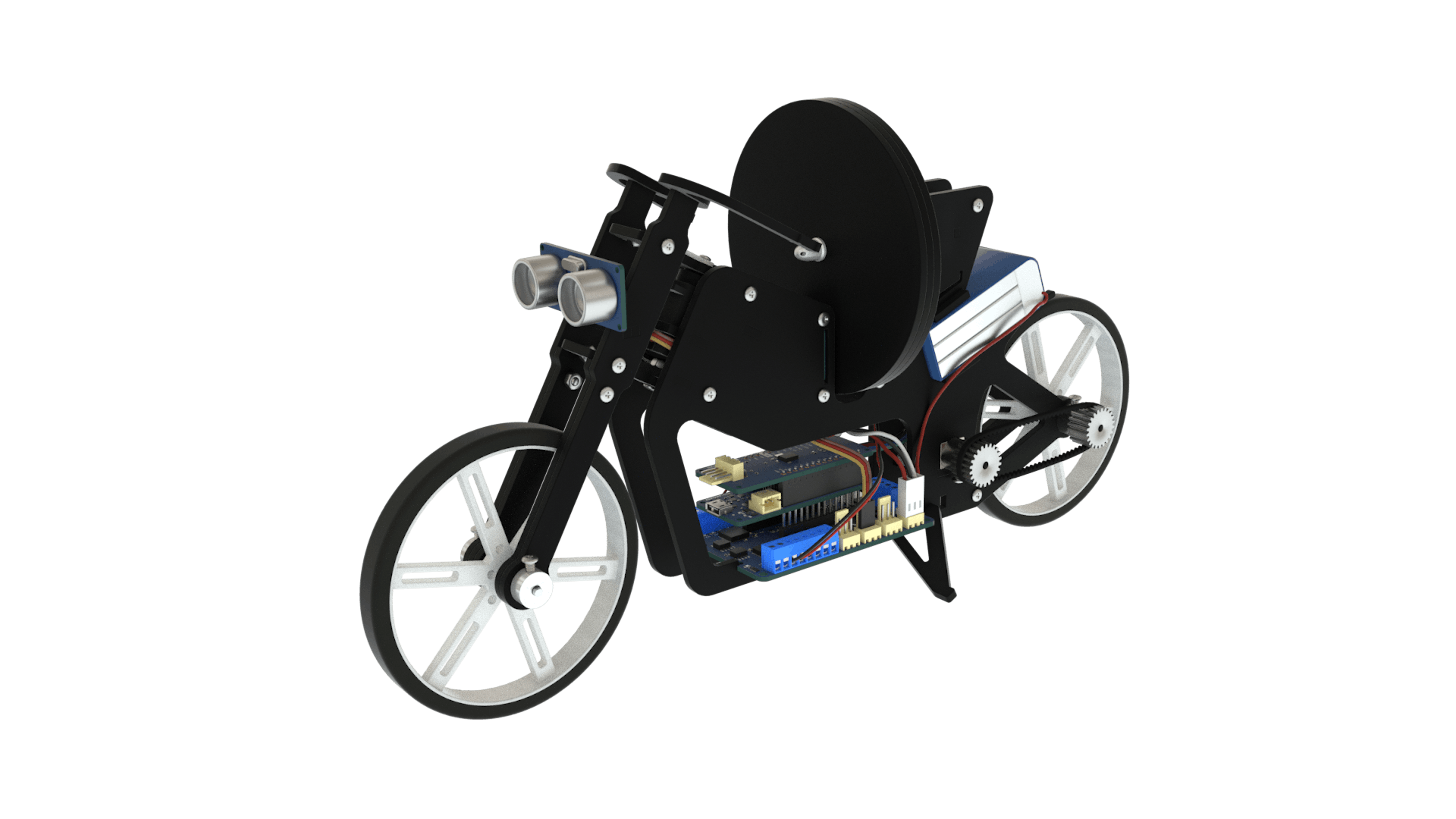
The motorcycle project consists of a two-wheeled robot that can balance and move using a rotating disc, which we will call inertia wheel from now on, to compensate if the motorcycle loses balance. The motorcycle is controlled by an Arduino MKR1000, the Arduino MKR Motor Carrier, a DC motor to move the back wheel, an encoder, a DC motor to control the inertia wheel, a 6 axis IMU, a standard servo motor to steer the motorcycle’s handle, a distance sensor, and a tachometer. In this project, you will learn how to simulate the vehicle’s overall behavior and create models to program the hardware components and improve the quality of the control algorithms. You will also explore how to program the motorcycle with Simulink®, control its balance algorithm, make it move in a straight line, and detect obstacles. After completing the project, you will have the knowledge needed to build your own self-balancing motorcycle, and who knows, maybe you’ll design yet another Hoverboard® or even the next Arduino-controlled Segway®. Before you begin modeling, you will need to assemble the motorcycle by following the instructions at
In the exercises that make up this project, you will learn how to do the following:
-
Exercise 1: Model vehicle and learn how to simulate its behavior
- Introduction to the different tools; in particular, the Simulation Data Inspector that will help you display and compare signals between simulations.
- PID controllers applied to controlling the angle at which the motorcycle leans
-
Exercise 2: Understand sensors & actuators and use Simulink and Arduino to program these
-
Exercise 3: Build a balance control algorithm using the Simulink models that you developed for the different hardware components
-
Exercise 4: Learn how to balance the motorcycle when it follows a straight line
-
Exercise 5: Balance the motorcycle while steering and using the lean angle to your advantage
EXERCISE 1:
6.1 Model vehicle and simulation
The motorcycle is a vehicle which controls balance via an inertia wheel system which is controlled by implementing a Proportional-Derivative (PD) controller. In this exercise, you will learn how to use different tools to create a simulation of the motorcycle’s movement and develop an algorithm that will balance the vehicle in a variety of external conditions.
In this exercise, you will learn to
- Understand the physical dynamics of the motorcycle-inertia wheel system.
- Identify the control terms in a PD controller and understand their respective effects in a closed-loop control system.
- Use a Simulation Data Inspector to monitor and refine a system simulation
- Develop a control algorithm to balance the motorcycle.
UNDERSTANDING MOTORCYCLE EQUATIONS OF MOTION
Let’s begin by understanding the equations of motion for the motorcycle-inertia wheel system. In the derivation below, we will examine a simplified version of the system, so you can create a functioning simulation that is not too complex.
We will make the following assumptions:
- The motorcycle is free to move only about the wheel-ground axis.
- There is no rotational friction between the motorcycle and the ground or between the motorcycle and the inertia wheel.
- The motorcycle wheels’ thickness is negligible.
- Air resistance is negligible.
Let’s have a look at a diagram that shows the coordinates that we will be referencing, along with important physical quantities:
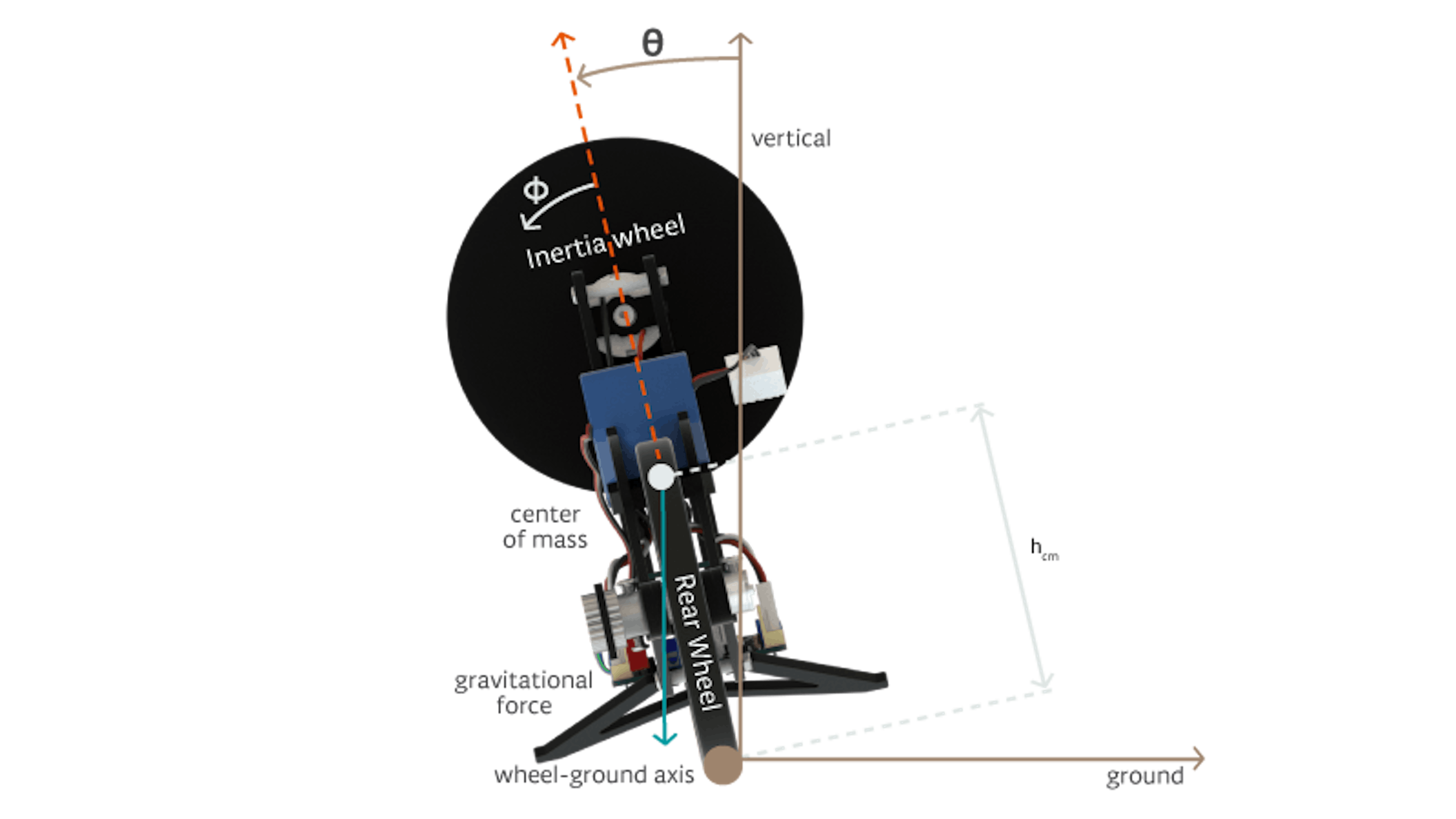
To help you understand this diagram, imagine that you are looking at the motorcycle from behind. You may want to place the motorcycle in front of you in this orientation as you read through the description as it will help you more readily understand the physics of the project. The most important coordinate shown here is the lean angle, θ, which is equal to 0 degrees when the motorcycle is perfectly upright, positive when the motorcycle leans counterclockwise when viewed from behind, and negative when the motorcycle leans clockwise. Another important angle is the rotational displacement of the inertia wheel, φ. As the inertia wheel rotates relative to the rest of the motorcycle, φ varies in value, where positive displacement is defined as counterclockwise.
Next, find the center of mass of the entire motorcycle system (including the inertia wheel). This location can be measured experimentally in the laboratory, but it is approximately just below the inertia wheel. The center of mass location is important to the dynamics of the motorcycle because the gravitational force acts directly through this point. The height of the center of mass from the ground when the motorcycle is upright (θ = 0) is defined as $h_c$$_m$
The motorcycle system is free to rotate around the wheel-ground axis, which is an imaginary line that connects the points on the rear and front wheels where they touch the ground (into the picture). The inertia wheel can rotate along its own axis, which goes directly through the middle of the inertia wheel.
Now let’s think about the torques in the motorcycle system. In a system that is free to rotate along an axis, a torque occurs when a force is exerted on the system at some point of the rotational axis. The magnitude of the torque can be determined by using the following equation:
$\tau$ = $|F \cdot r\cdot \sin(\alpha)|$
In this equation, the torque, $\tau$, is expressed in units of force ∗ length (e.g., Newton-meters). F is the force being exerted, r is the distance between where the force is applied and the axis of rotation, and $\alpha$ is the angle measured at the force exertion point between the force direction and the axis of rotation. According to the equation, the maximum torque is achieved when the force is applied at a right angle (90 degrees). The torque is zero, when the force is applied directly toward or away from the axis of rotation. Furthermore, you can get more torque with the same force if the force is applied farther from the axis of rotation.
For a given axis of rotation, there is a net torque, which is the sum of all torques acting on the system about that axis. The net torque is proportional to the angular acceleration of the rotating system:
$\tau_{sys} = \sum_{i}\tau_{i,sys}=I_{sys}\ddot\theta_{sys}$
In this equation, $\tau_{i,sys}$ denotes the torque applied to the system about the rotational axis. Isys is the moment of inertia of the system with respect to the rotational axis. The moment of inertia is a property of a rigid object that measures the mass distribution of the object with respect to a rotational axis. $\ddot\theta_{sys}$ is the angular acceleration of the object about the rotational axis.
Now let’s consider the motorcycle system, which includes the rear and front wheels, the steering column, the motorcycle body (along with all its embedded electronics), and the inertia wheel. The axis of rotation for this system is the wheel-ground axis, and the measure of rotation is the lean angle θ, defined earlier.
The torque acting on the motorcycle (denoted with M) about the wheel-ground axis has 3 major components:
- Gravitational torque $(\tau_{g,M})$
- Inertia wheel torque $(\tau_{IW,M})$
- External torque $(\tau_{ext,M})$
The gravitational torque is due to the gravitational force pulling down on the center of mass of the motorcycle system when it is not directly above the wheel-ground axis (i.e. when it is leaning). Using the first equation from above, the gravitational torque can be found as follows:
$\tau_{g,M} = M_M \cdot g \cdot h_{cm}\cdot sin(\theta)$
In the above equation, $M_M$ is the mass of the motorcycle system, g is the constant gravitational acceleration, $h_c$$_m$ is the height of the center of mass from the wheel-ground axis, and θ is the lean angle. In this equation (and all subsequent equations in this chapter), a positive torque value is defined to be in the counterclockwise direction with respect to the understood rotational axis. You can see that there is zero gravitational torque when the motorcycle is perfectly upright (θ = 0). For a small lean angle θ, a small gravitational torque is exerted on the motorcycle in the same direction as the lean. As the angle gets larger, the torque increases until the motorcycle falls 90 degrees. If this were the only torque acting on the motorcycle, the motorcycle system would have an unstable equilibrium at θ = 0. This means that any small perturbation of the motorcycle from its equilibrium will cause the system to accelerate away from its equilibrium position rather than move back towards it.
However, we have other torques in the motorcycle system to prevent it from falling! When the inertia wheel motor is actuated, the motor shaft will exert a torque on the inertia wheel, causing it to accelerate (rotationally). The inertia wheel will then exert an equal and opposite torque on the motor shaft due to conservation of angular momentum. Let’s call this reaction torque $\tau_{IW,M}$
The last type is external torque, $\tau_{ext,M}$. This torque encompasses all other torque sources acting on the system. This could include things like your USB cable pushing up against the motorcycle, air resistance, wind, and various other disturbances like pushing the motorcycle to the side with your finger. In this theoretical discussion, we will focus on the ideal scenario in which $\tau_{ext,M}$ = 0. Ultimately, you want your motorcycle to balance even when there is a reasonable amount of external perturbations acting on it.
Thus, we have the net torque on the motorcycle about the wheel-ground axis:
$\tau_{net,M} = I_M \cdot \ddot\theta = \tau_{g,M} + \tau_{IW,M} + \tau_{ext,M}\approx \tau_{g,M} + \tau_{IW,M}$
Here, $I_M$ is the moment of inertia of the motorcycle system about the wheel-ground axis.
Now let’s look at another rotational axis: the one that goes through the inertia wheel motor shaft. On this rotational axis, only the inertia wheel is free to rotate. The torques acting along this axis are from the DC motor, which we will call $\tau_{motor,IW}$, and from dissipative forces like friction between the moving parts and drag effects, $\tau_{fric,IW}$. We will assume that there is no such mechanical resistance in this system, or $\tau_{fric,IW}$ = 0. Using the same torque definition, we have the following equation:
$\tau_{net,IW} = I_{IW}\ddot\phi = \tau_{motor,IW} + \tau_{fric,IW} \approx \tau_{motor,IW}$
Here, I$_I$$_W$ is the moment of inertia of the inertia wheel with respect to its central axis, and $\ddot\phi$ is the angular acceleration of the inertia wheel. You will have direct control over $\tau_{motor,IW}$ when you actuate the inertia wheel DC motor through the MKR1000 board.
Next, let’s put it all together. Recall the torque that the motor shaft exerts on the inertia wheel is equal and opposite to the torque that the inertia wheel exerts on the motor shaft and thus, the rest of the motorcycle. Or,
$\tau_{IW,M} = -\tau_{motor,IW}$
Substituting into the equation for $\tau_{net,M}$ we have:
$\tau_{net,M} \approx \tau_{g,M} - \tau_{motor,IW}$
$I_M \cdot \ddot\theta \approx M_M \cdot g \cdot h_{cm} \cdot \sin(\theta) - \tau_{motor,IW}$
The motion of the inertia wheel is defined by:
$I_{IW} \cdot \ddot\phi = \tau_{motor,IW}$
We now have the dynamics of the lean angle expressed in terms of measurable constant quantities (i.e. masses, lengths, and moments of inertias). The question now is “What should $\tau_{motor,IW}$ be so that the motorcycle stabilizes at θ = 0?” We will explore this question throughout this chapter and the project.
For now, let’s examine the simplest possible corrective torque that may turn the unstable equilibrium point into a stable equilibrium point. Suppose the lean angle is very small (perhaps a few degrees). The following approximation holds for small values of θ (when measured in radians):
$\sin(\theta) \approx \theta$
We then have a simpler approximate differential equation for the lean angle:
$I_M \cdot \ddot\theta \approx M_M\cdot g\cdot h_{cm}\cdot\theta - \tau_{motor,IW}\sin(\theta) \approx \theta$
Now, suppose we program the motor to exert a torque that is proportional to the lean angle itself:
$\tau_{motor,IW} = K_p\cdot\theta$
Here, K$_p$ is a constant whose optimal value may be determined via simulation and experimentation. Substituting into the previous equation, we have:
$I_M \cdot \ddot\theta \approx -(K_p - M_M\cdot g\cdot h_{cm})\theta$
If K$_p$ is greater than $M_M \cdot g \cdot h_{cm}$, then the angular acceleration of the motorcycle about the wheel-ground axis is in the opposite direction of the lean angle. Specifically, when the motorcycle leans one way, it will accelerate in the opposite direction. When the motorcycle moves to the other side of the equilibrium point, the angular acceleration will then switch directions to move the motorcycle back toward equilibrium. This is a stable equilibrium, which means when the system is perturbed from the equilibrium position, it will restore itself back toward equilibrium.
Solving the differential equation, we have a solution of the form:
$\theta(t) = A\sin(\sqrt{\frac{K_p - M_M \cdot g \cdot h_{cm}}{I_M}}t + B)$
In the above equation, A and B are constants that depend on the initial values of θ and θ˙. If you increase the constant K$_p$, the oscillation frequency becomes faster. In this ideal scenario, in the absence of any perturbing torques, the motorcycle system will oscillate about the vertical position with constant amplitude forever. This is known as proportional control and is often a first attempt at developing a control algorithm to bring a system to some desired state. We will want to improve this behavior so that the oscillations decay in amplitude and eventually settle to a constant lean angle of 0 and the motorcycle system responds stably when random perturbations act on it. In the following section, you will use Simulink to model these dynamics.
PHYSICAL MODELING IN SIMULINK
First Test: Torque-Free Inertia Wheel
Once you understand the equations that govern the motorcycle’s dynamics, the next step is thinking about possible ways to implement a control mechanism that will, given the parts available in the kit, balance the motorcycle vertically. Let’s look at a Simulink model that implements the motorcycle’s physical behavior, as described in the previous section. Open the model by typing the following in MATLAB Command Window:
Since you will modify the model, save it as myMoto.slx.
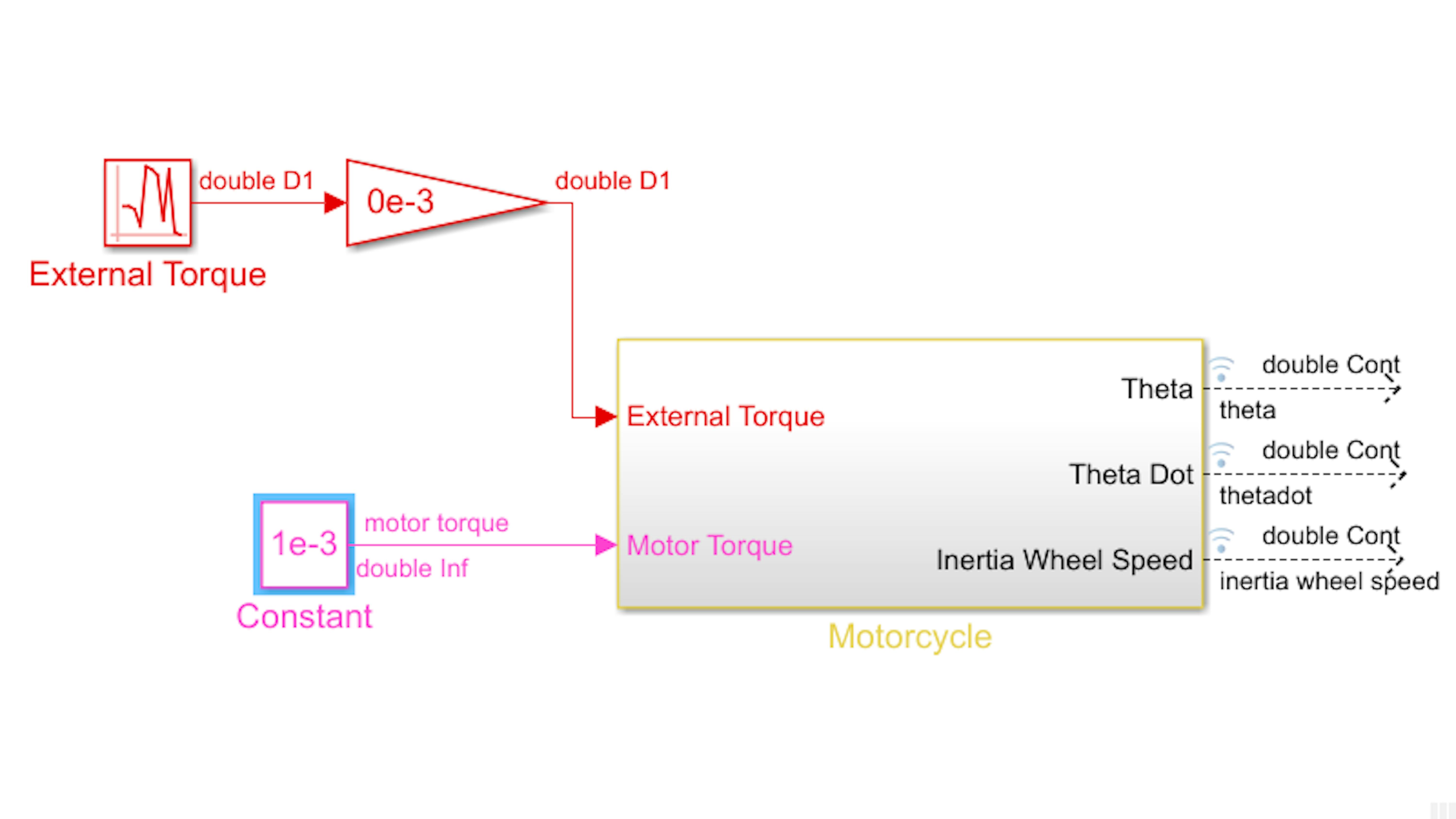
The model contains a Motorcycle subsystem block, External Torque block to generate a data array, Gain block that is a signal multiplier, and a Constant block to provide data input.
>> motoSys0_start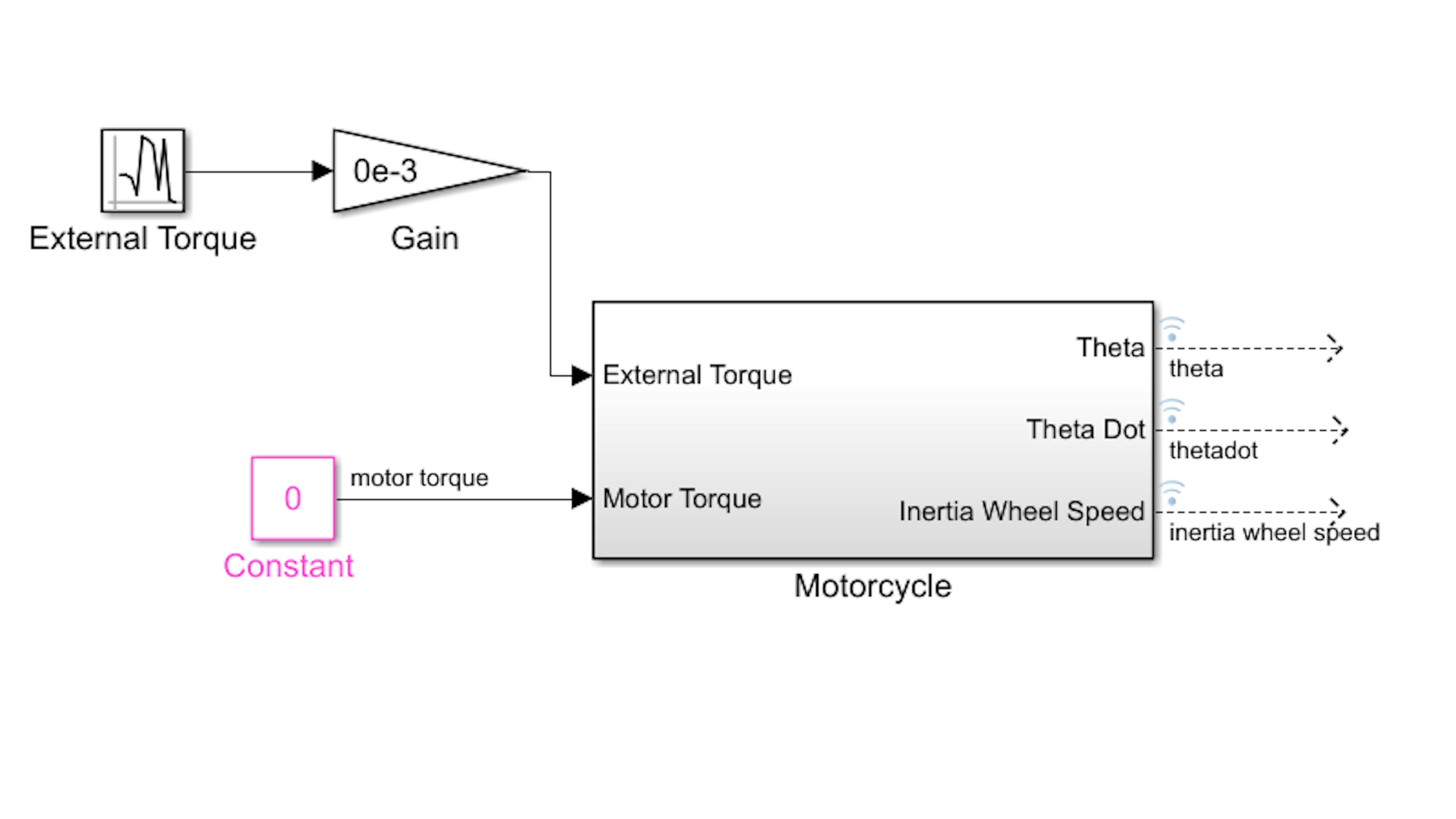
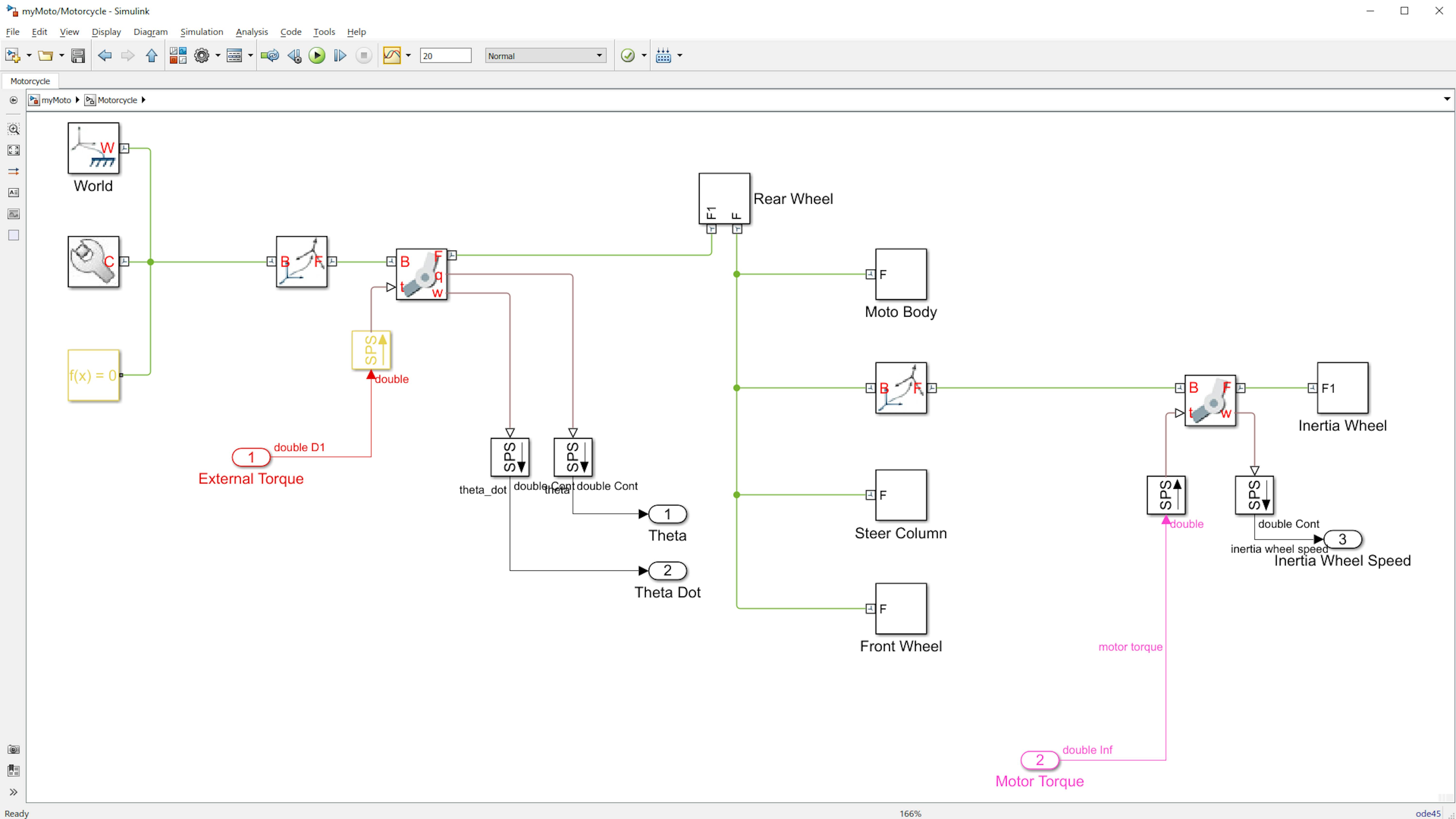
Let's examine the Motorcycle subsystem by double clicking on it:
Notice the inputs to the subsystem are an external torque from the environment and a torque applied to the motorcycle by the inertia wheel motor. The model inside the subsystem generates the physical quantities of interest: the lean angle θ, its time derivative $\dot\theta$, and the time derivative of the inertia wheel angle, $\dot\phi$.
The physical dynamics of the motorcycle are modeled here using Simscape Multibody™. This is a part of the Simscape™ modeling software package and enables you to simulate and animate multi-component systems in which physical masses are connected by geometric constraints. Notice in this subsystem there are colored signals with no arrows. These are Simscape signals and unlike Simulink signals which represent unidirectional data flows, these signals represent physical connections between components. The blocks that connect to these Simscape signals represent physical components and rotational and translational transforms between them and various reference frames. Notice that there are blocks for each of the 5 independently movable parts of the motorcycle: the motorcycle body, the rear and front wheels, the reaction wheel, and the steering column. These blocks contain the component geometries, masses, moments of inertia, and reference coordinates for each of the 5 parts. Finally, Simulink-PS Converter and PS-Simulink Converter blocks let you convert Simscape signals to and from Simulink signals, so that it can interface with the rest of the model.
Let’s have a look at the Revolute Joint block connected to the Rear Wheel component. The Revolute Joint block defines a rotational axis of motion between two solid components in the model. Double click the block and expand State Targets:
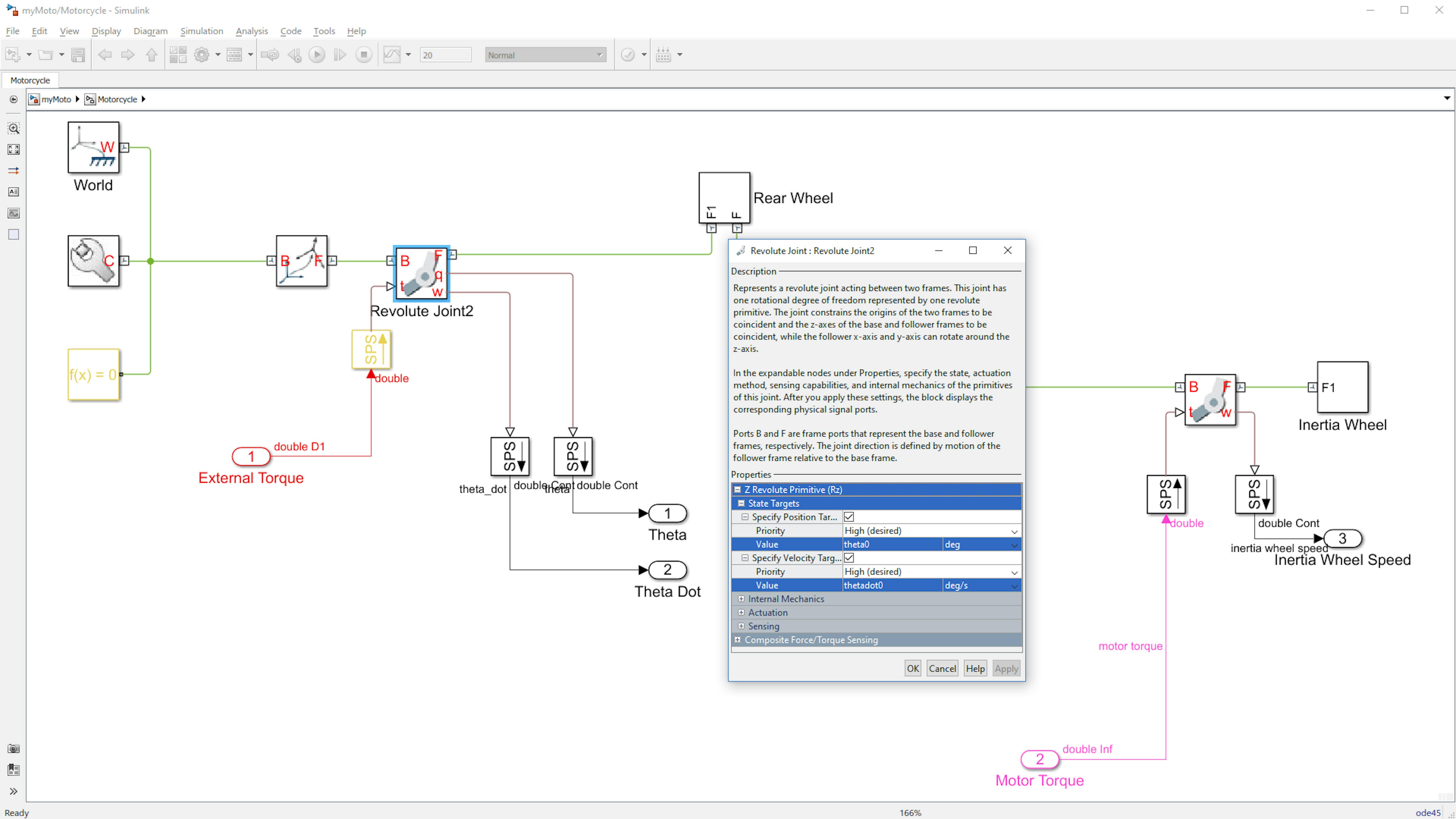
This is where the initial conditions are specified for the lean angle and its time derivative. They are stored in MATLAB variables theta0 and thetadot0, respectively. Similarly, the initial angle and angular speed of the inertia wheel are stored in the Revolute Joint block next to the Inertia Wheel component.
Let’s see how the motorcycle behaves when no external torque and no motor torque are applied. Run the model and watch the Simscape Multibody animation when it pops up in the Mechanics Explorer window. The following image displays a frame of the simulation:

In the animation window, you will see a 3D model with different objects represented in different colors. We have prepared the models in terms of the independent moving parts in the motorcycle: the front and rear wheels, the steer column, the motorcycle body, and the inertia wheel. Underneath the animation window, there is a simple scrollbar that can be used to control the animation’s playback. On the top-right part of the animation window, there is a series of buttons that can be used to zoom, pan, and change the viewing angle. Take a few moments to experiment with the playback and perspective buttons until the motorcycle is fully visible in the viewing frame.
The simulation window has a full physics engine that can simulate gravity. Without any help from the inertia wheel motor, the motorcycle simply rotates about the wheel-ground axis, oscillating about the downward direction due to gravity. You can observe that the model contains no physical “ground” and continues revolving right through where the ground would be. Although it is possible to model hard stop boundaries using Simscape Multibody, it is beyond the scope of this material and instead we will focus our attention on the behavior of the system when the motorcycle lean angle is close to zero.
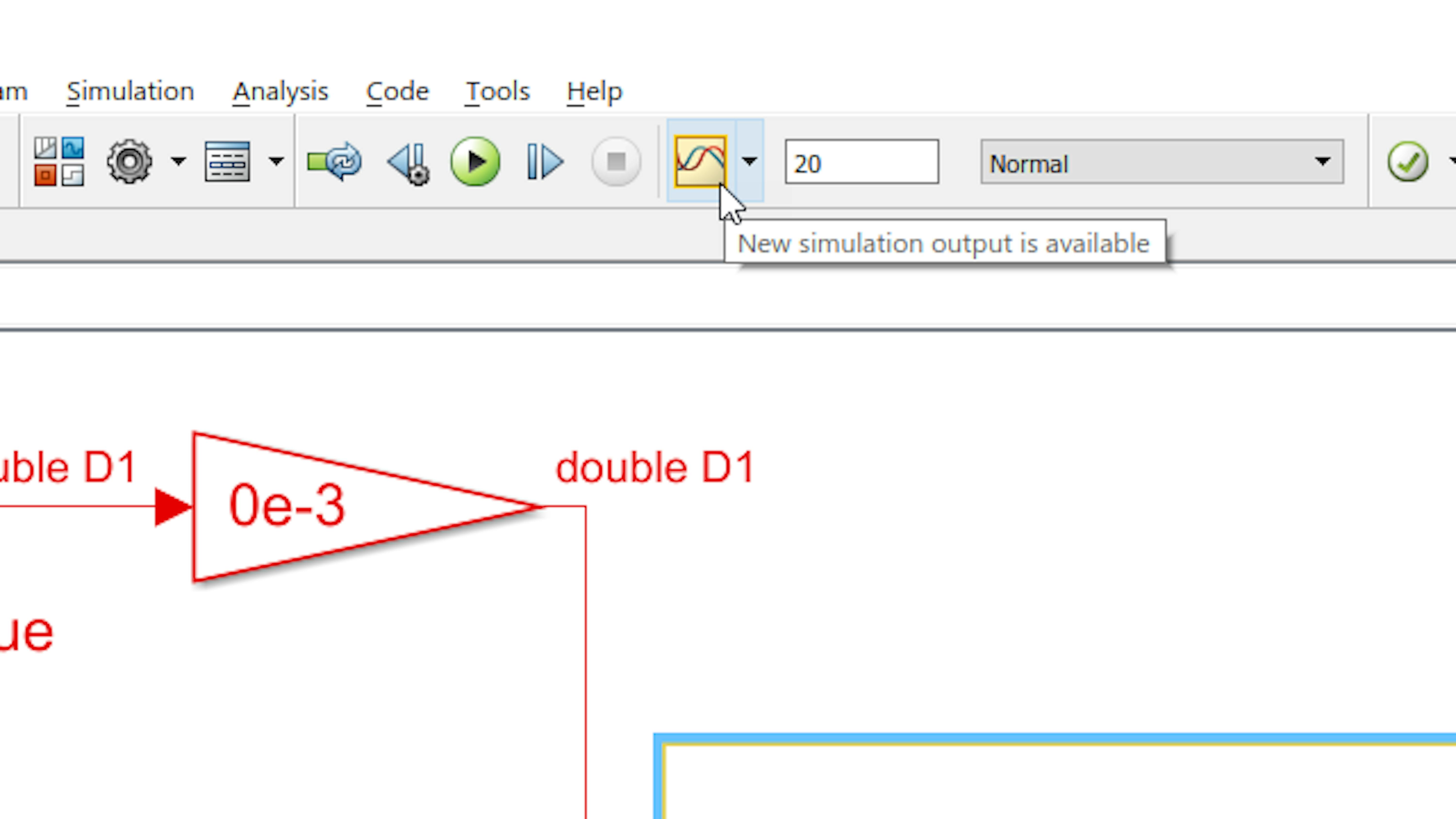
Next, let’s take a quantitative look at the motorcycle’s behavior. Go back to the model window and click on the Simulation Data Inspector button in the Simulink toolstrip as highlighted in the following image:
Selecting this button will open the Simulation Data Inspector (SDI) window. SDI is an environment where you can view logged data from simulations, examine them in any combination of graphical axes, and compare the same signals across multiple simulations. You will use SDI to observe the behavior of the motorcycle system and fine-tune your control algorithm to optimize performance.
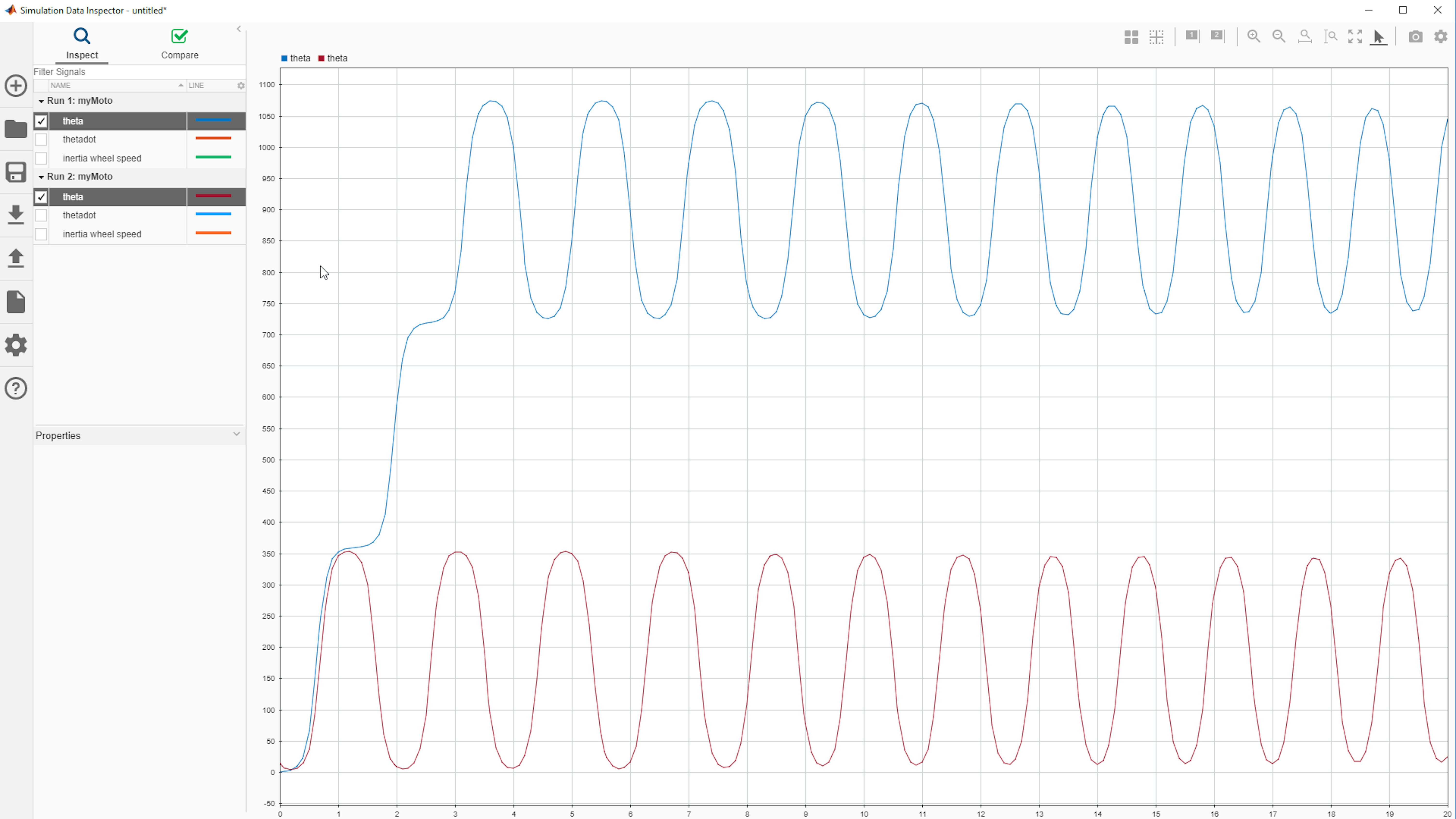
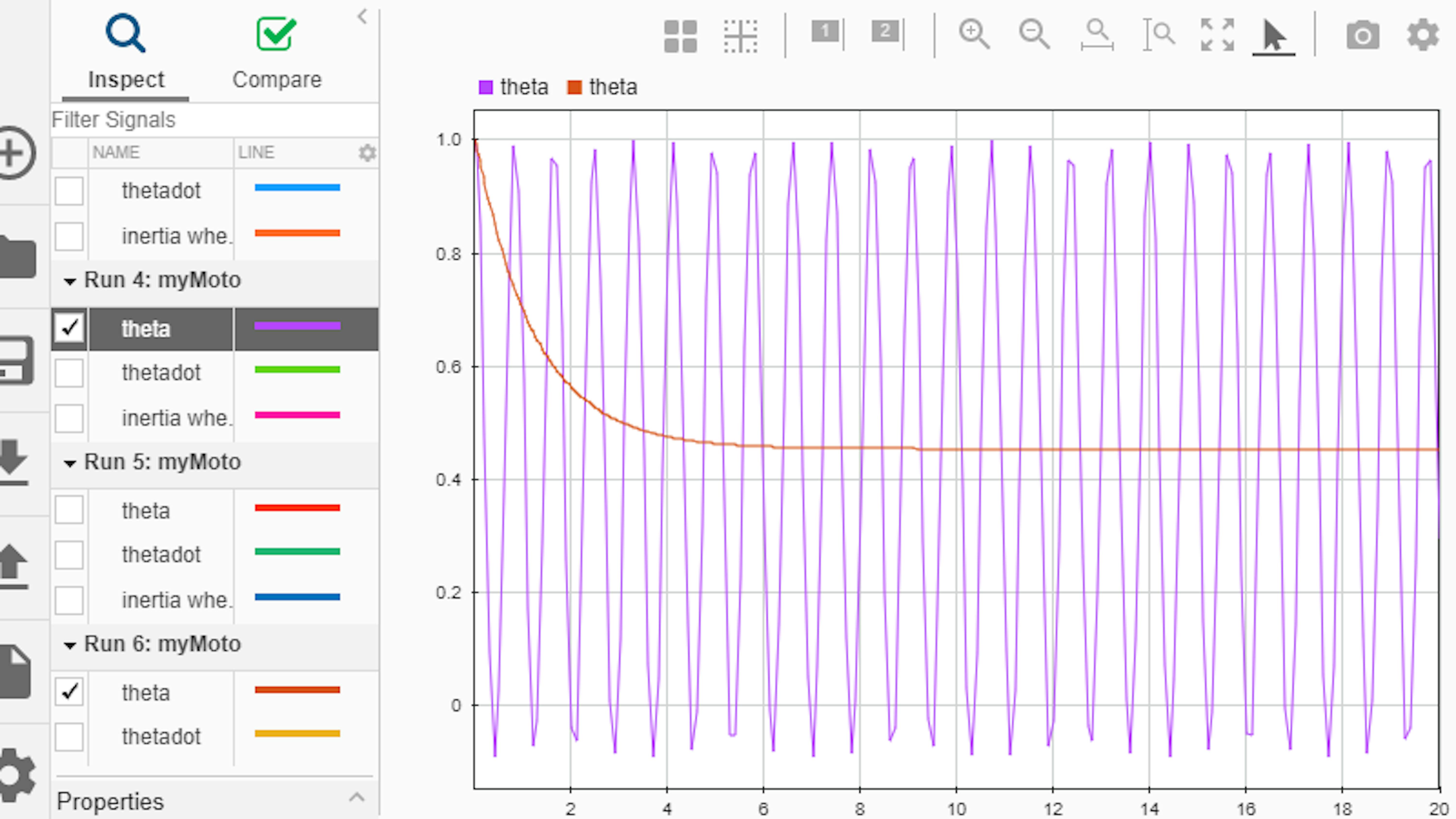
In the SDI window, select theta and thetadot from the list of available signals and observe them on the graphical axes. If you remember the view of the Motorcycle block, there were just three outports: theta, thetadot, and inertia wheel speed. The next image shows the results of this operation for our simulation:
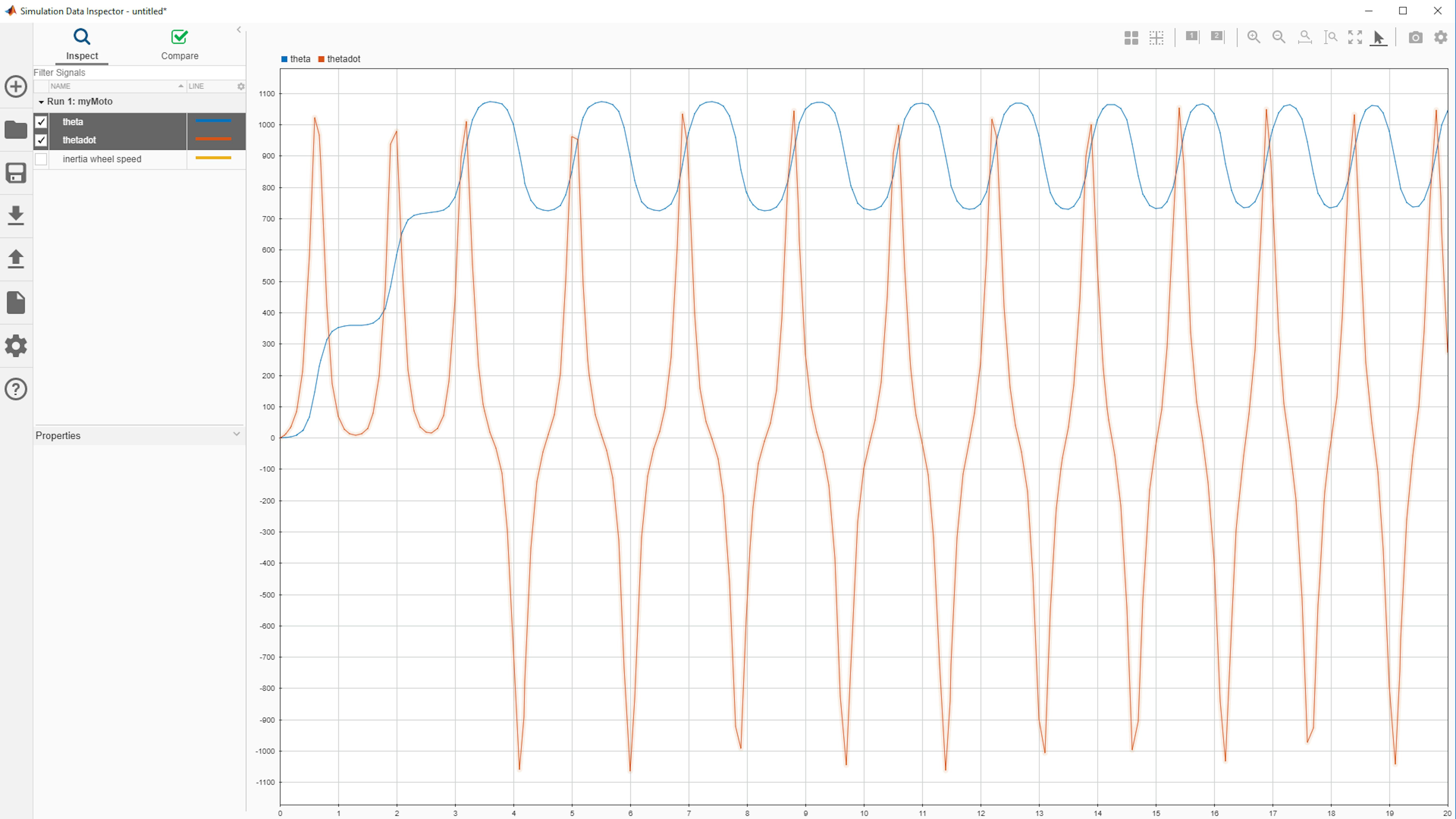
You will notice that the signals present an oscillatory behavior. You can see the signal properties on the bottom left; click on one of the signals to choose which one will be presented.
Unselect the angle measurements and select the inertia wheel speed checkbox to see its behavior on the screen:
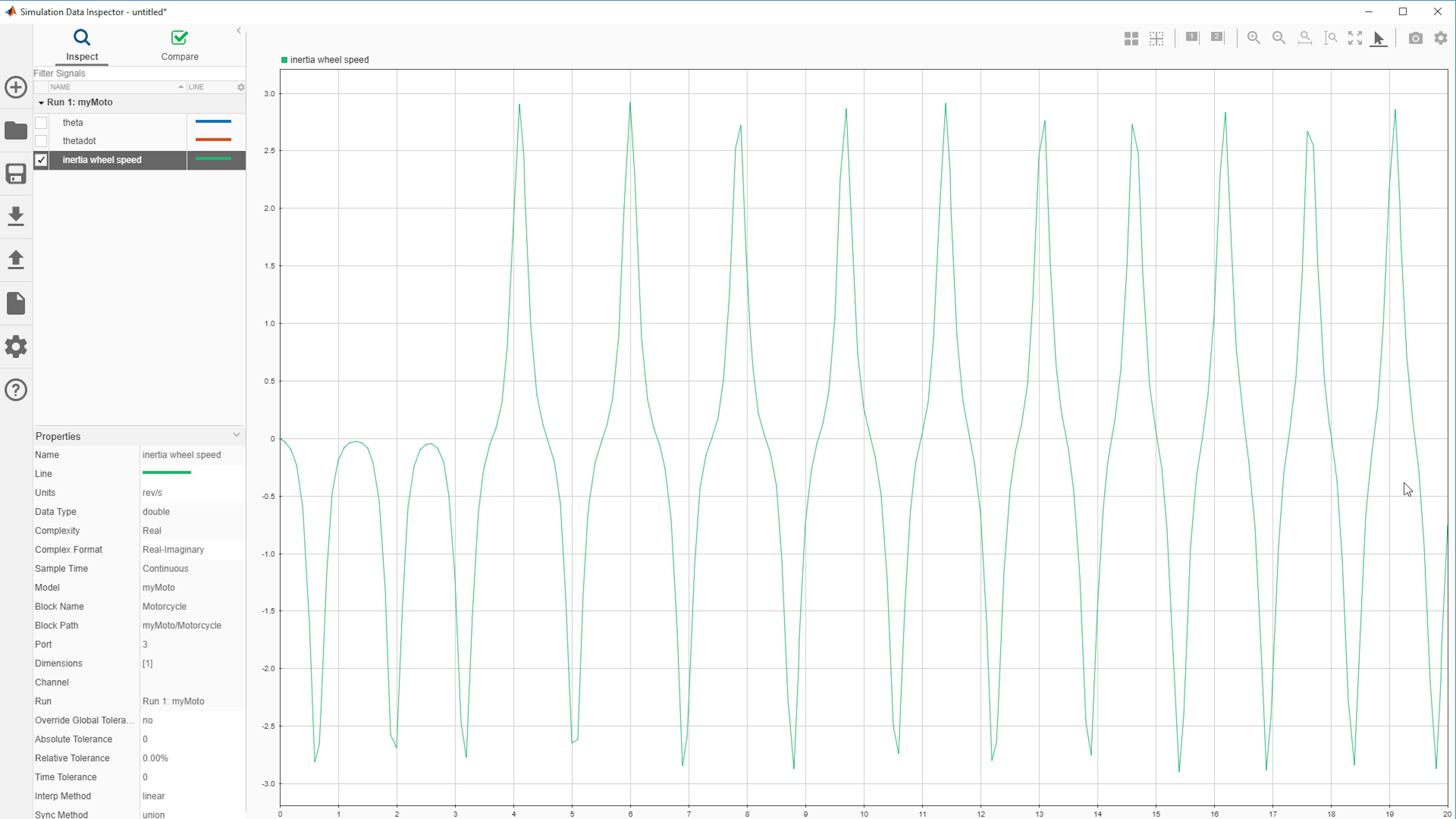
Notice how the inertia wheel oscillates in response to the motorcycle’s motion about the wheel-ground axis. Its shape shows the same oscillatory behavior (same frequency and similar shape -but inverted- to thetadot) we observed.
To further explore how the model behaves, you need to change the initial conditions. Set the initial conditions as follows by typing the following commands in MATLAB
>> theta0 = 15;
>> thetadot0 = -135;
Run the simulation and watch the animation. What happened this time? Can you figure out the relationship between the initial angle conditions and the motorcycle’s behavior in the animation? To make sense of it you should observe the new data in the SDI window and compare it to the data collected from the previous simulation. The following image shows how the first run of the simulation needed some time to reach a steady-state where the theta signal enters a purely oscillatory state versus the second one, where the signal is, directly in that state:
Try experimenting with different initial conditions and examine their effect on the modeled behavior. More importantly, check the simulation to see what happens to the motorcycle. Remember that you are checking a situation when the inertia wheel is not applying any torque, which is not how the motorcycle will behave in the real world.
Second Test: Adding Motor Torque
Now, let’s experiment with motor torque on the inertia wheel. For this test, you will have to first set the initial conditions as follows
>> theta0 = 1;
>> thetadot0 = 0;
Go to the top level of the myMoto.slx model and set the value in the Constant block to 1e-3:
Observe the effect on the lean angle (theta) and the inertia wheel speed when compared to the first run:
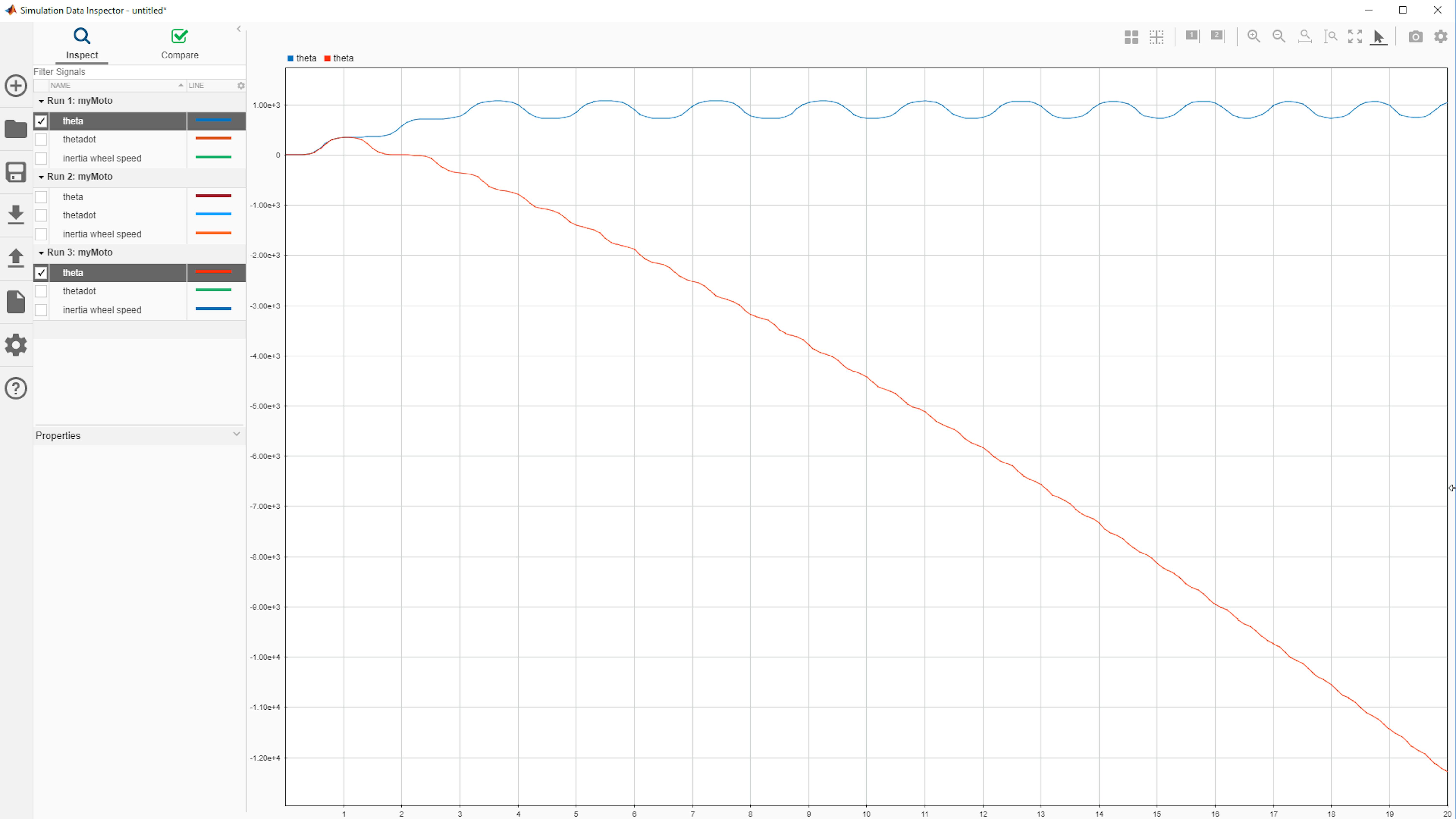
The lean angle continues to oscillate but now has an added component that makes it decrease at a constant speed. In the real world, this means that the Motorcycle will fall, but since there is no “ground” as such in the model, the motorcycle will start to rotate around its horizontal axis.
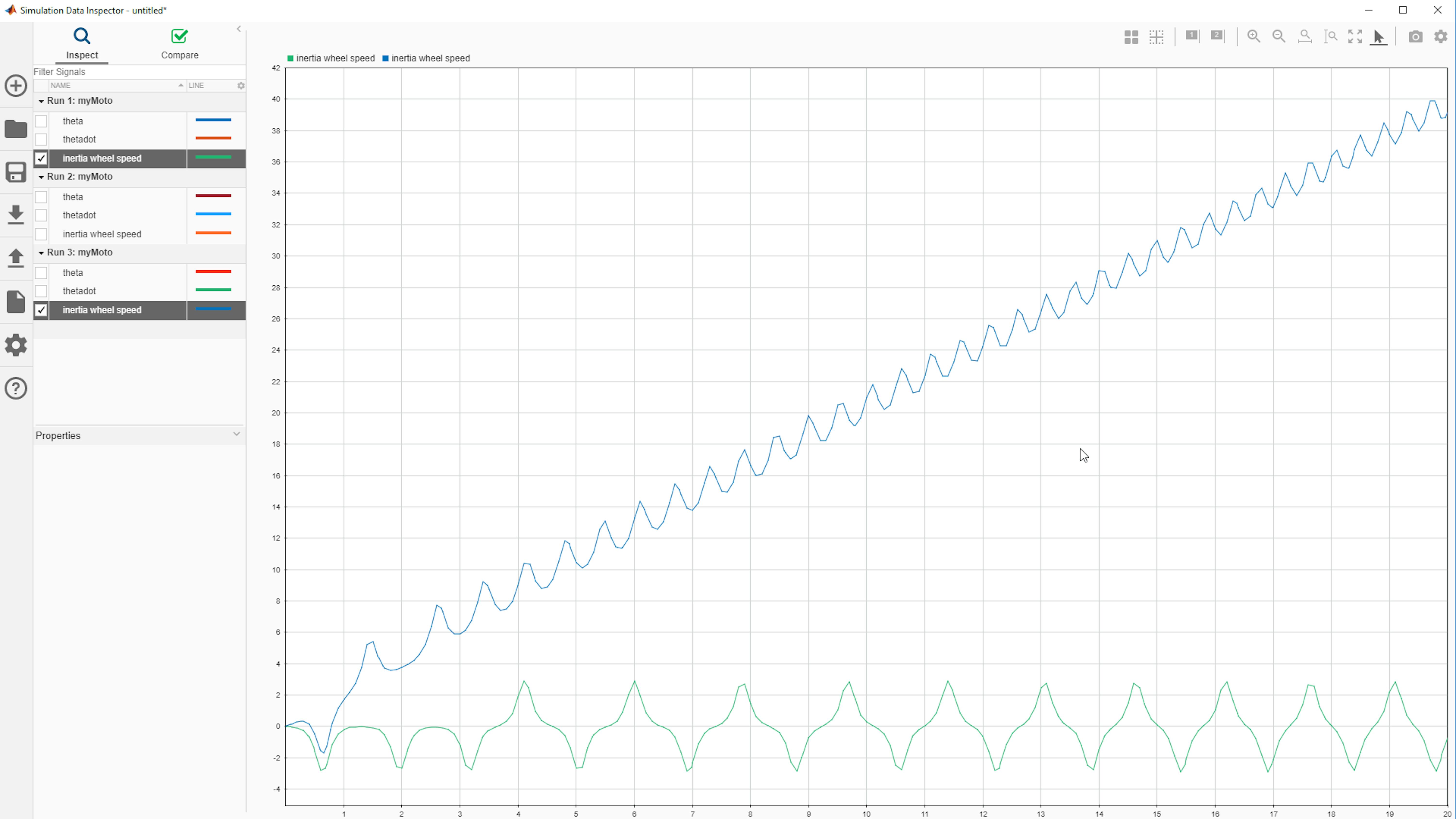
As you can see, the average speed of the inertia wheel increases indefinitely. This is not possible in the real world since the motorcycle will break at some point: either the motor will stop its acceleration because of mechanical conditions or the motor driver will break because of over-current. While neither of these situations is desirable, it is uncertain which will happen first (i.e. mechanical or electrical damage). Therefore, we need to design a controller so that the motorcycle will never reach such a state.
Designing a Controller for Balance
Let’s add some torque to the inertia wheel. To help keep the motorcycle balanced, we need to figure out how to use some of the information we are collecting from theta and thetadot so that we can compensate for the gravitational torque acting on the motorcycle. In terms of the equations derived earlier, we want to always keep θ (theta on the model) close to zero to balance the motorcycle. The most straightforward way to balance the motorcycle is to apply a torque that is proportional and opposite to θ. To do this, the motor needs to apply a proportional torque to the inertia wheel in the same direction as θ.
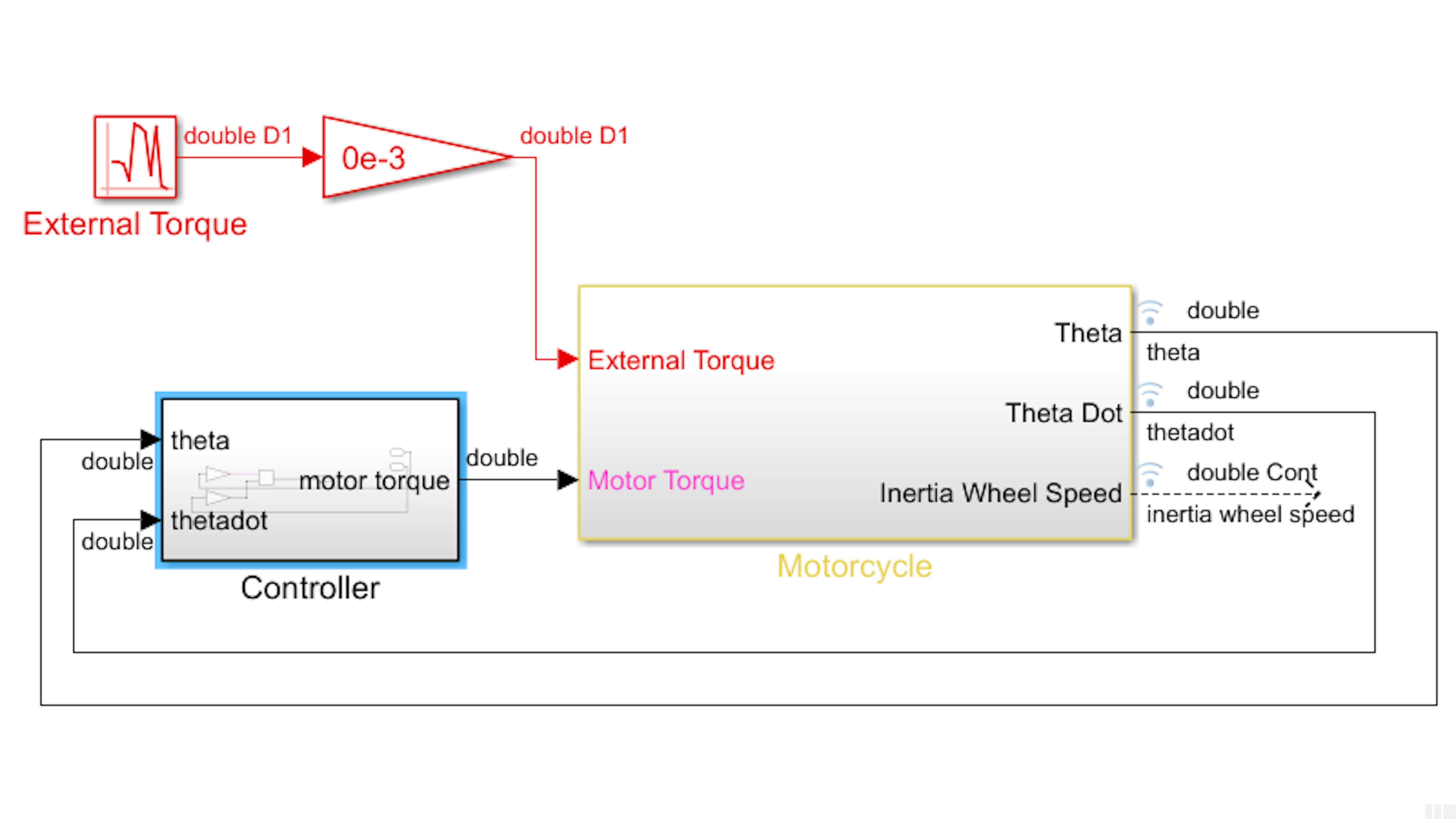
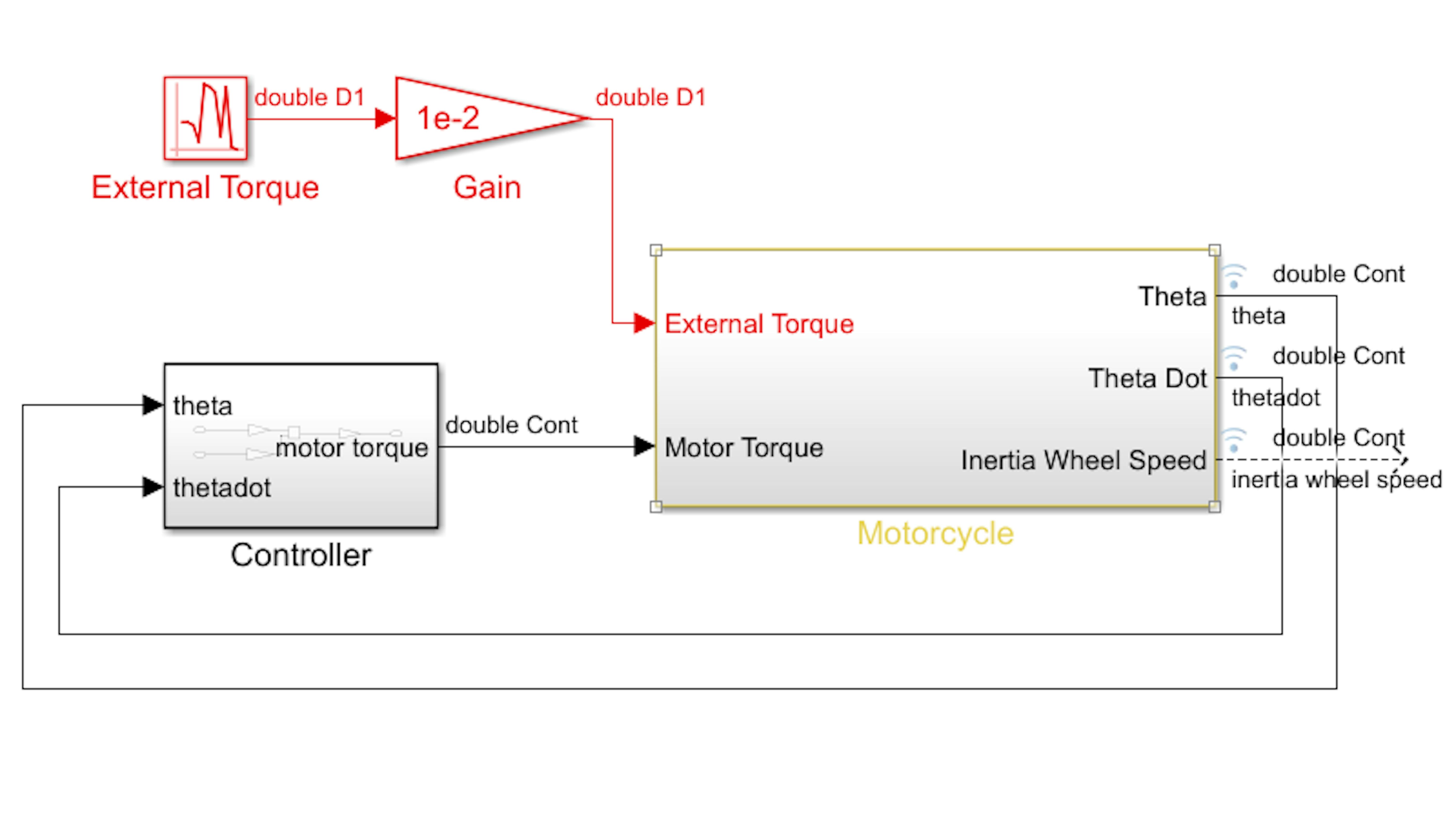
Starting from the last model (myMoto.slx), delete the Constant block and add a Gain block. Set the gain value to 1e-2. Connect and label the gain block as shown in the following figure, where you can see how we use theta to affect the Motorcycle block:
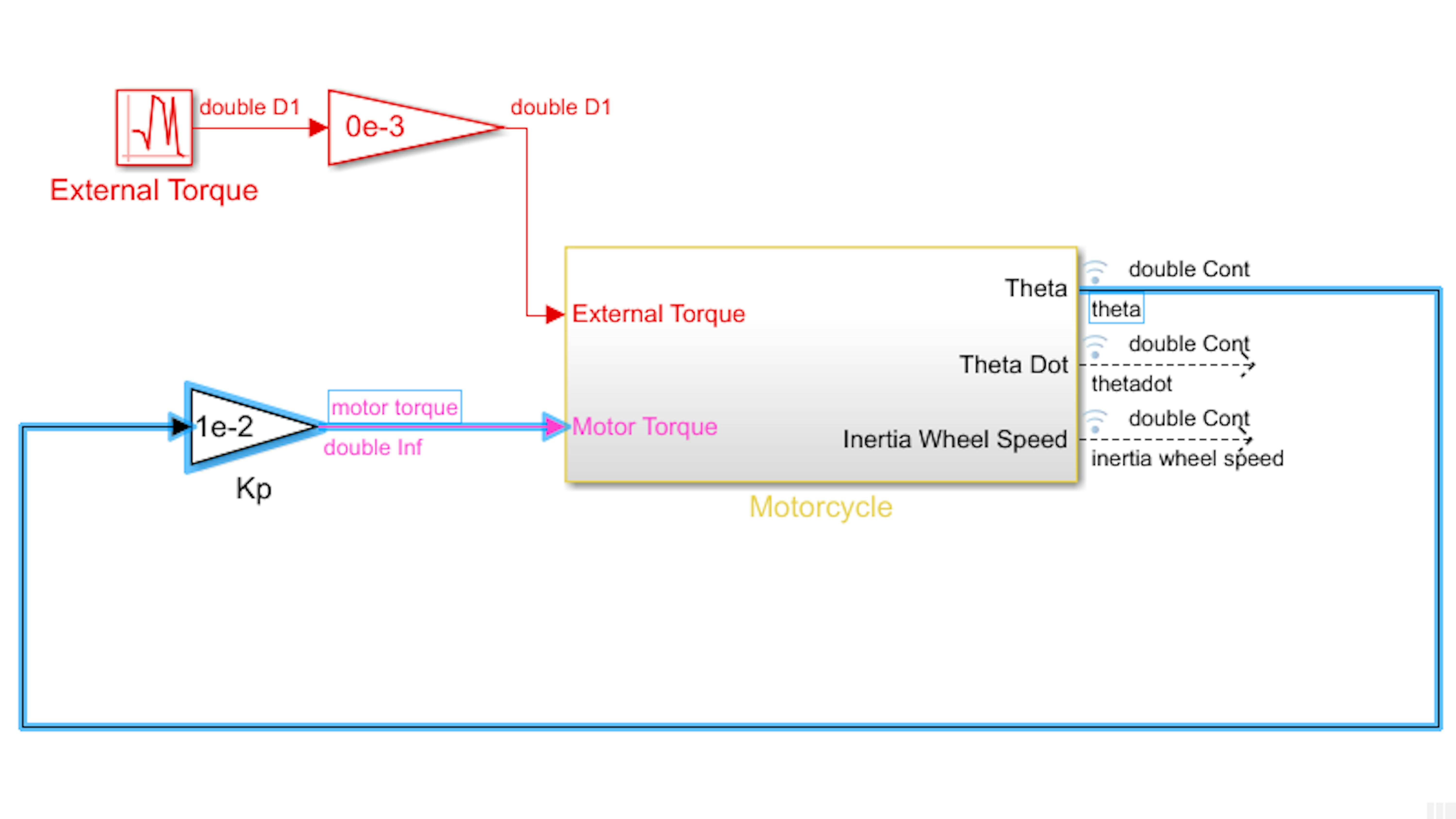
We have labeled the Gain block as $K_p$ to signify that this is a classic proportional control (the “P” of PID); as you can imagine from here we are going to develop an argument about how the proportional component works and why it is convenient to add other parts to it to create a better mechanism of control of the wheel. Run the simulation and watch the animation in the Mechanics Explorer window. What are your observations regarding the stability of the motorcycle and the oscillatory behavior? Examine the signal theta in the SDI window for this last simulation:
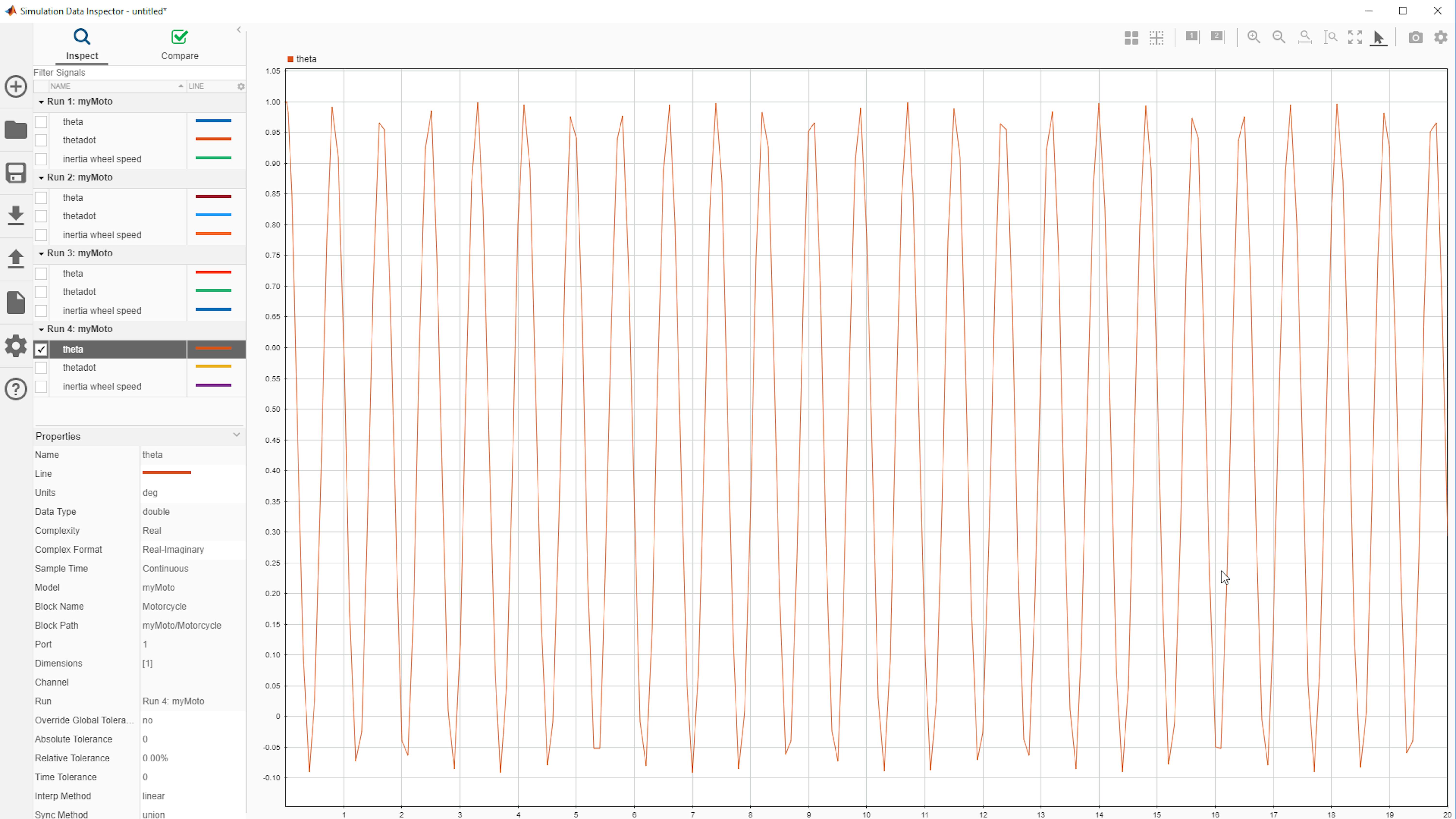
Now, try running the simulation with different values of the gain and examine theta in the SDI window. In the following image, we applied a value of 2e-2 and you can see how both the frequency and amplitude of theta are affected:
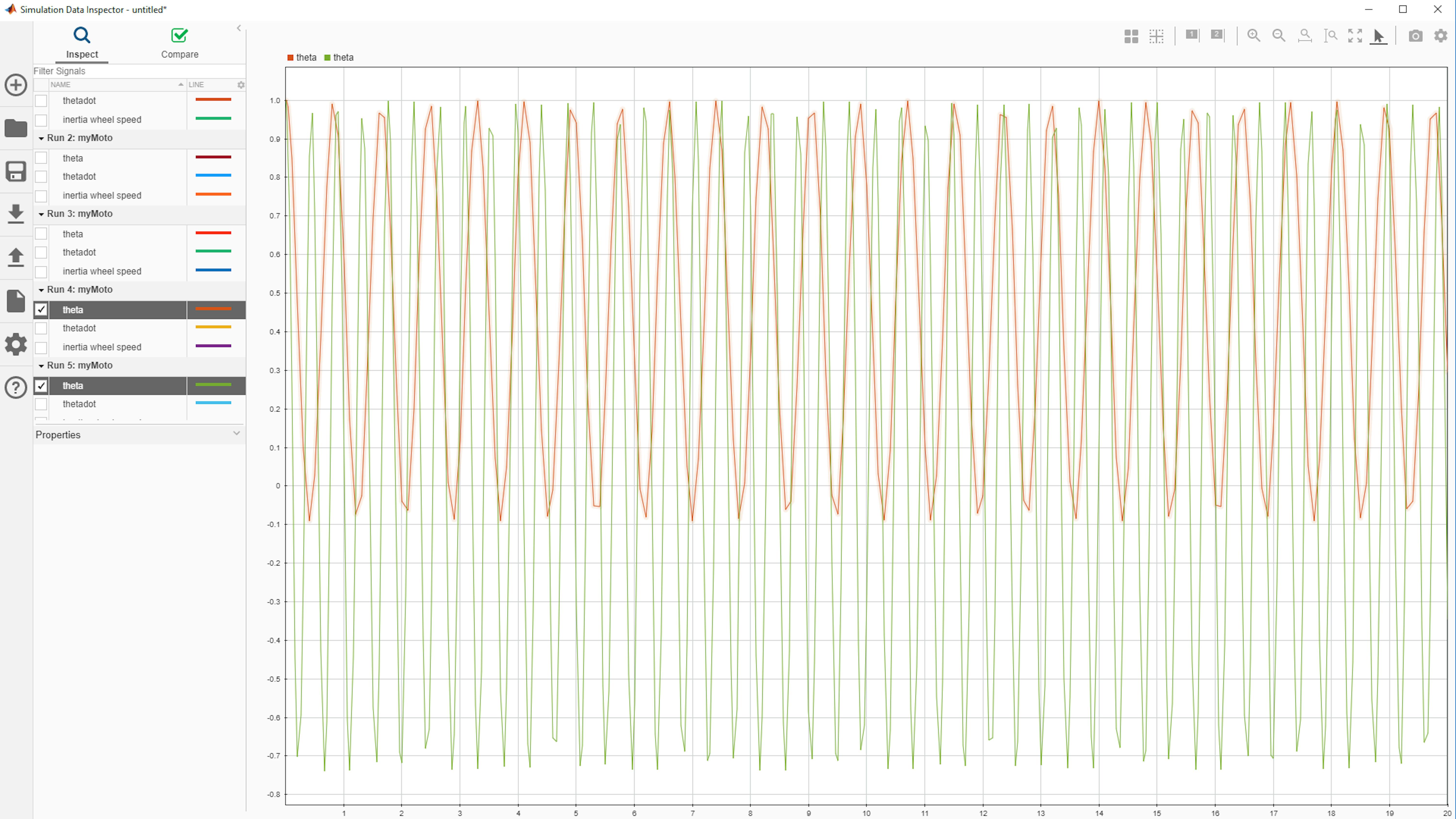
What happens to theta when the proportional gain is increase and decreased? What happens if the proportional gain is set too high or too low?
As per our earlier derivation, you should observe that increasing the proportional gain causes the oscillatory frequency to increase, and the amplitude of oscillation to also increase. If you set the gain too low, there will not be enough torque from the motor to keep the motorcycle balanced against the gravitational torque. If the proportional gain is set too high, the motorcycle will overcompensate and push too far past the center of balance, causing a fall.
Find a value for the proportional gain that stably balances the motorcycle and set it in the $K_p$ Gain block. Run the simulation to get a set of baseline data into SDI; we will use this data later as a reference while improving the design of the controller.
Decreasing the Oscillation in Your Controller
The controller Kp = 1e-2 is stable, but theta oscillates about the desired lean angle with constant amplitude indefinitely. Let’s modify the control algorithm so that the oscillations in theta dampen over time. To do that, you not only need to counteract the lean angle, but you also need to counteract the angular rate of the lean angle.
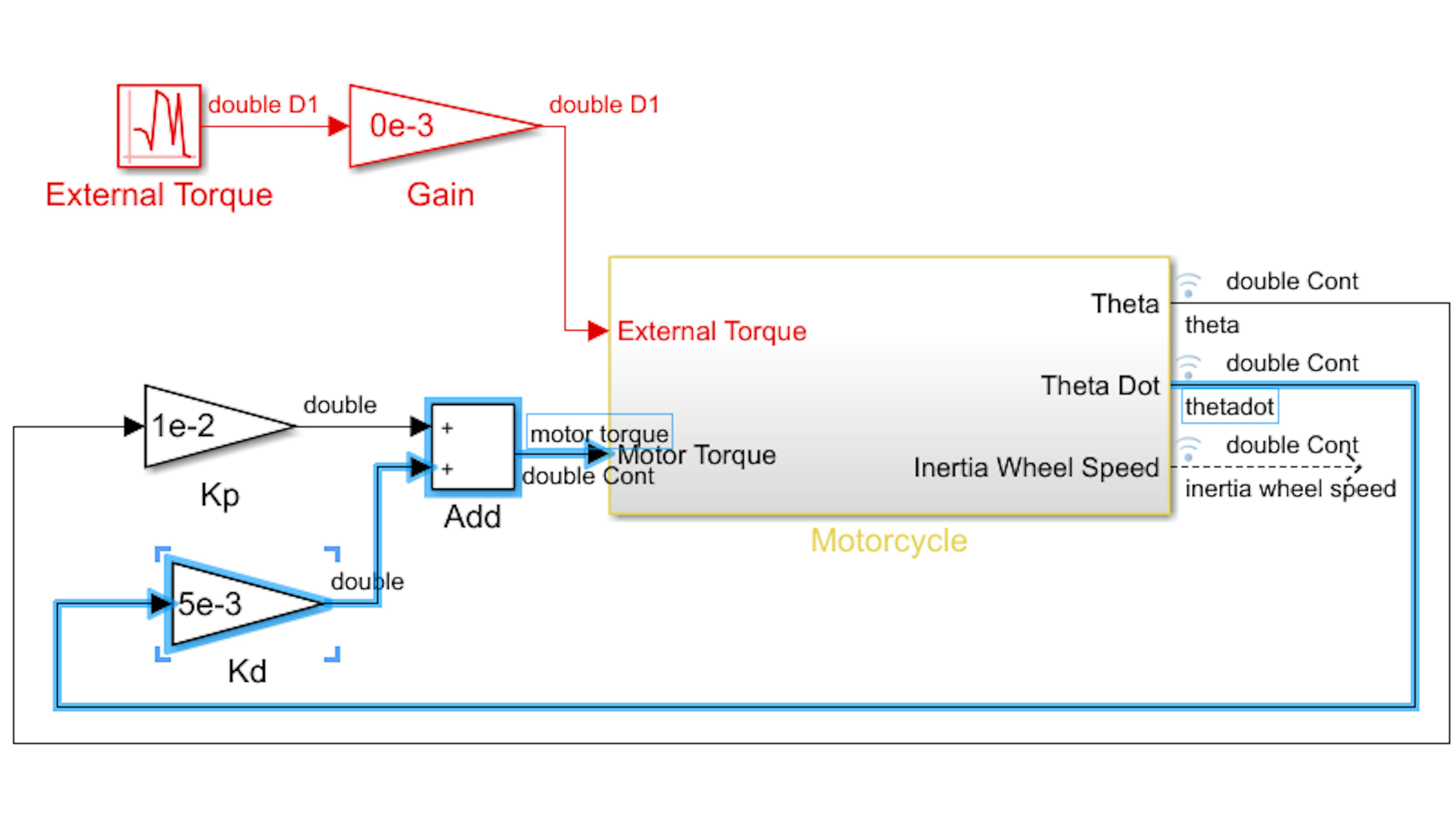
Add another Gain block and an Add block to the model. Set the gain value of the new Gain block to 5e-3. Label the new Gain block “Kd” as it will be introducing the derivative term of the PID controller. Make the connections so that the final configuration looks the same as the following schematic:
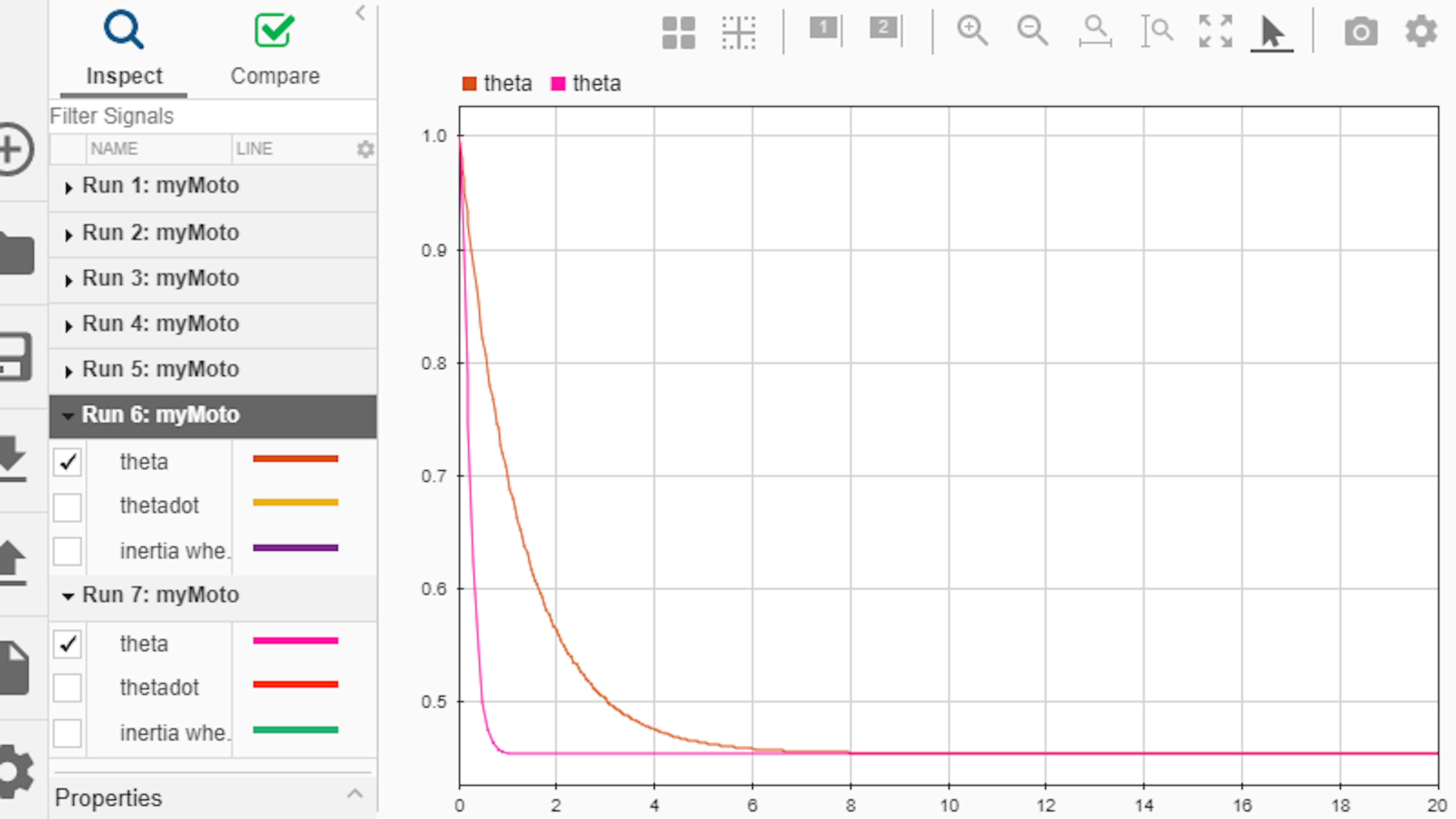
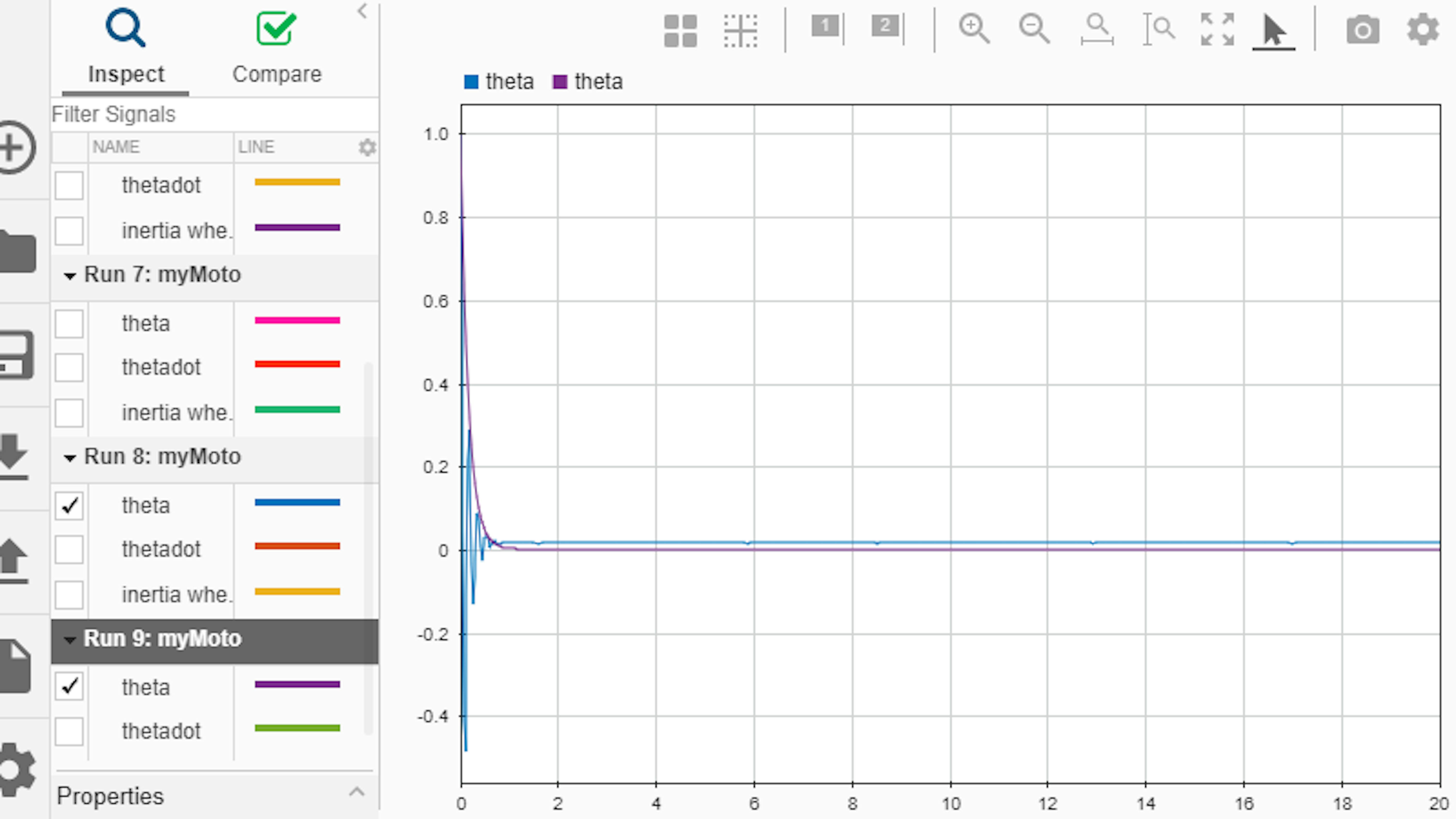
Run the model and watch the animation. Then examine theta in the SDI view and compare it to theta from the previous run:
How does the derivative gain impact the oscillations in theta? As you can see, the oscillatory behavior is now eliminated or “damped” over time, making theta become constant and thus, reaching a steady state. You should ask yourself whether the steady state value of theta (close to 0.5 in the above image) is desirable. Would we not want this variable to reach a state of equilibrium? If you think about it, once the motorcycle has reached the perfect vertical position (theta = 0), you don’t need to keep the inertial wheel accelerating since there is no external force to compensate against. However, if the steady state is reached before the motorcycle has reached the vertical position, stopping the acceleration of the wheel is not such a good idea. Note that the steady state is reached having theta at a constant value different from zero, which means that the motorcycle will not be in balance. To summarize, we want the system to reach a steady-state of zero in a certain amount of time (not too soon, not too late).
Before focusing on compensating the steady-state error, experiment with the derivative gain. What happens to the oscillations in theta when the derivative gain is increased and decreased? What are the tradeoffs in lean angle behavior when the derivative gain is increased or decreased?
You will see that when the derivative gain is increased, there are fewer oscillations before the lean angle reaches a steady value, and the amplitude of oscillation decreases faster. When it is decreased, there are more oscillatory cycles, and it takes longer to reach a steady state. If the derivative gain is set too high, the motorcycle’s lean angle may change abruptly, which can cause it to become unstable. For the motorcycle’s balance controller oscillations in the lean angle are not desirable, but neither is having a large change in the lean angle over a short time.
Both the proportional and derivative gain can be tuned so that the system behaves as required when perturbed from the target state. Try different combinations of Kp and Kd gain values to see if you can achieve the desired behavior empirically.
As an exercise, let’s find values of the proportional and derivative gain which allows theta to stay within 0.05 degree of its steady-state value before 1 second has elapsed. The following SDI diagram shows what you should observe when you achieve this scenario (Kp = 1e-2 and Kd = 1e-3):
Eliminating Steady-State Error
Before the controller algorithm gets any more complex (and it will!), let’s create a separate subsystem. Highlight the two Gain blocks and the Add block, right-click on a selected block, and click Create Subsystem from Selection:
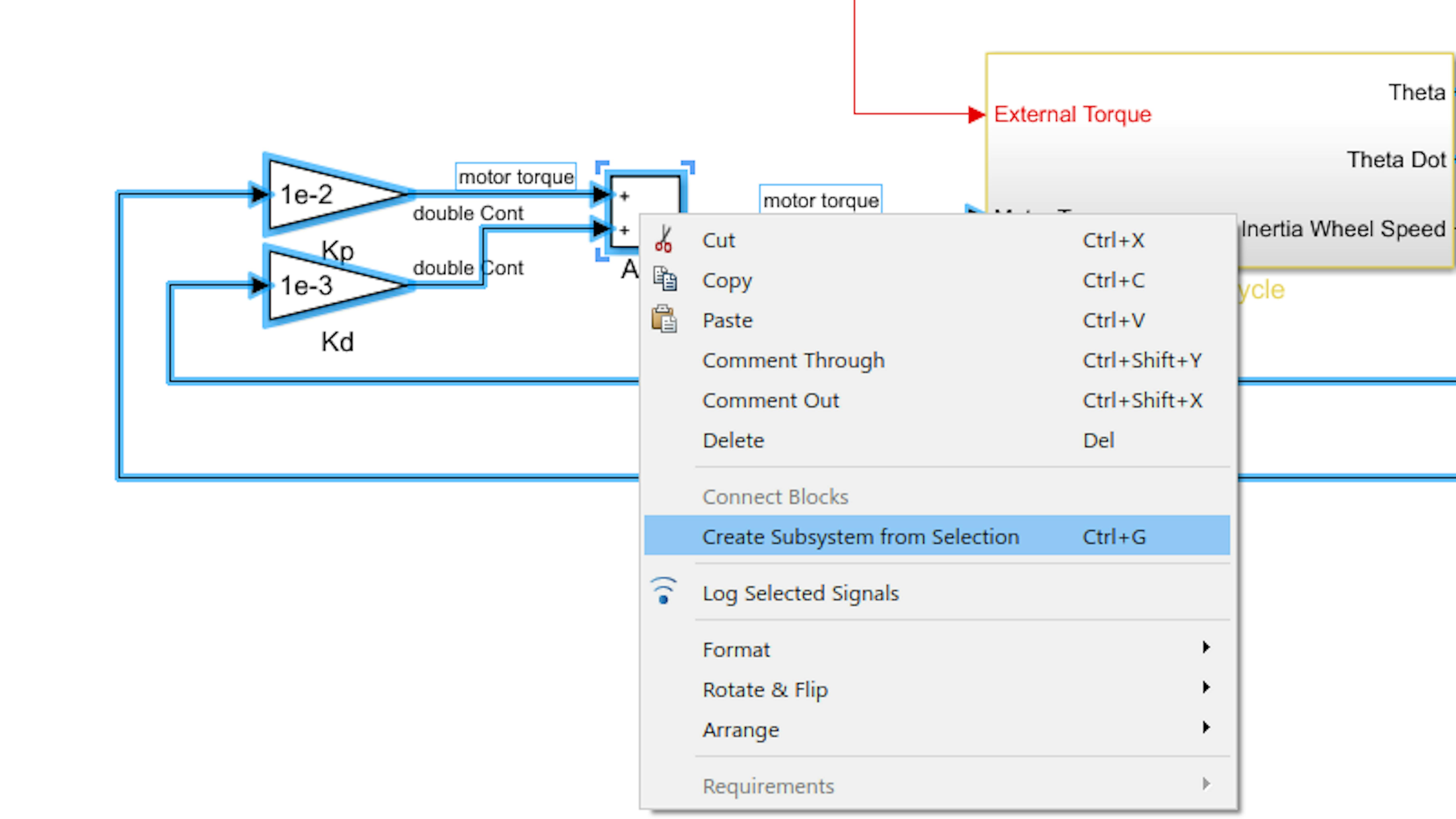
Name the Subsystem block “Controller” as shown:
Double click the controller block to go inside this new subsystem and rearrange the blocks to clean up the subsystem.
Now, let’s take care of the steady state error. A pure proportional-derivative controller, or PD controller, commonly suffers from steady state errors following a perturbation from the target state. You can resolve this by either increasing the proportional gain or by adding an integral term to the controller that counteracts the accumulation of errors over time. The accumulation of errors over time can be disadvantageous when you are trying to balance the motorcycle later. Because of this, we are going to use only the first approach of increasing the proportional gain.
Increase the Kp gain to 1e-1 and Run the model to watch the animation. Then examine theta in the SDI view and compare it to theta from the previous run:

Tune your PD (proportional-derivative) controller, with different values for the gains until you find a good compromise. The inertia wheel on your motorcycle should be able to help compensate the lean angle at a reasonable speed such that there are no oscillations on the lean angle.
For Kp = 5e-1 and Kd = 8e-2, you get the following theta curve which looks good.
Optimizing Parameters
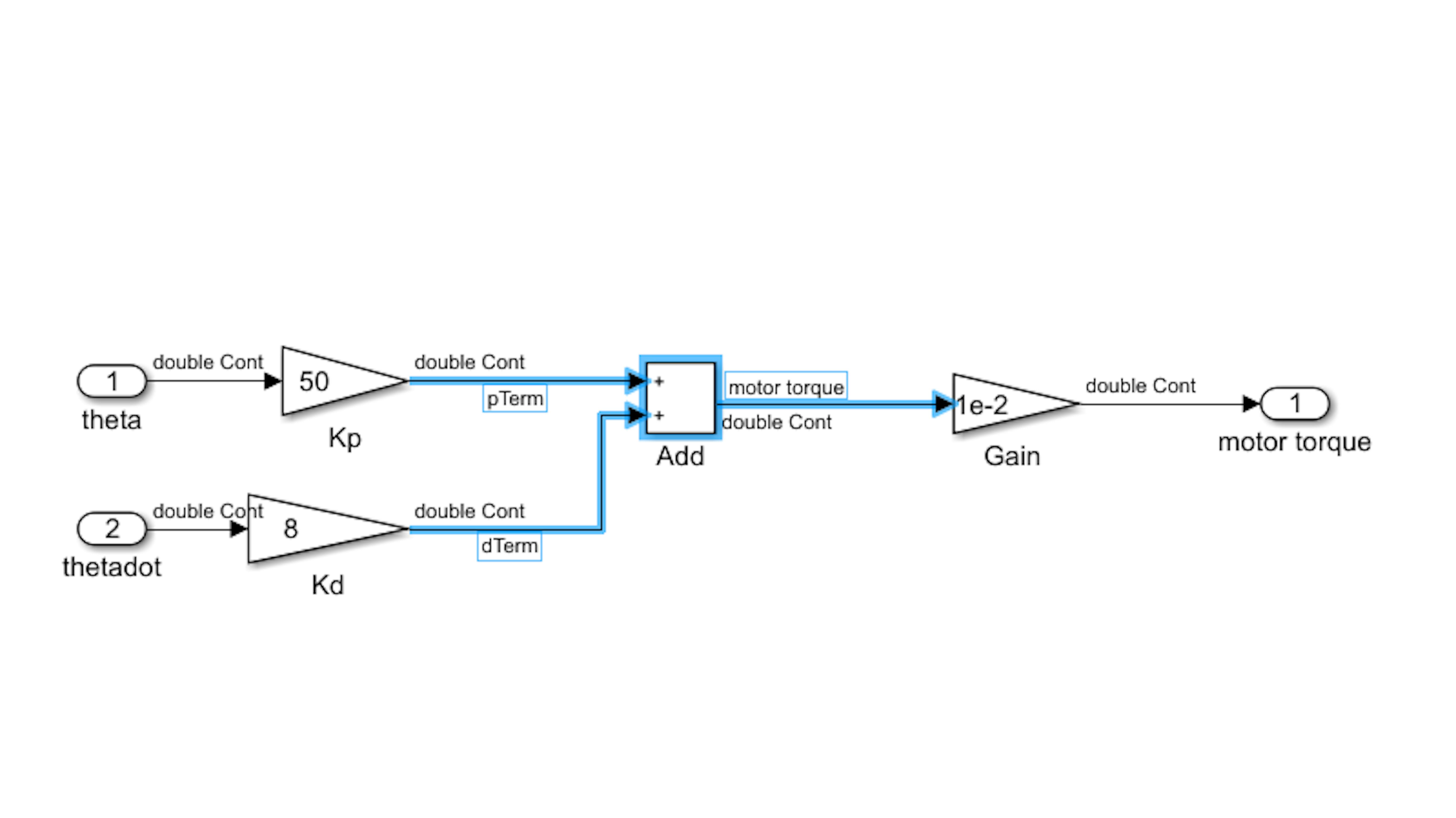
To simplify parameter tuning and prepare for a motor torque constant later, you can add an overall gain to the sum of the control terms. To do so, add a Gain block after the final Add block and set the gain value to 1e-2. Then, correct the Kp and Kd gain values by multiplying the existing values by 1e2:
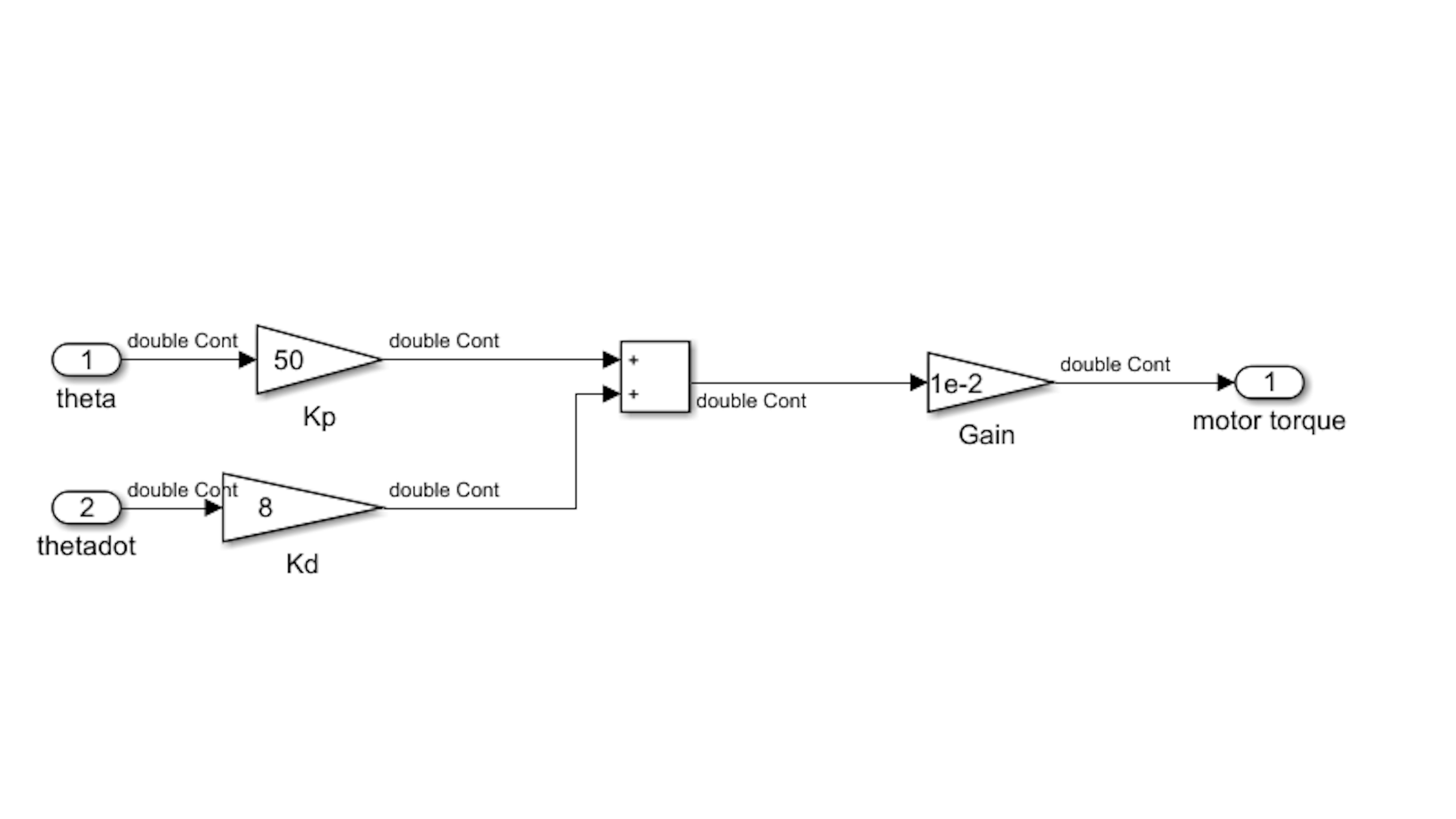
The configuration displayed in the previous image seems to be stable enough at this point. Furthermore, by adding the final multiplier, it is easier to play with the model when it comes to fine tuning the controller to respond to random variations of the torque.
Responding to Random Perturbations
Your PD controller works well under ideal conditions with the setup shown previously. The question is whether it will perform well with random perturbations. This is an extent that can also be modeled with MATLAB by adding a random noise, which you can do by setting the External Torque gain value to 1e-2, which will make the external torque input to the Motorcycle block more visible:
Run the simulation and watch the animation. Examine theta in the SDI view and compare it to the previous run:
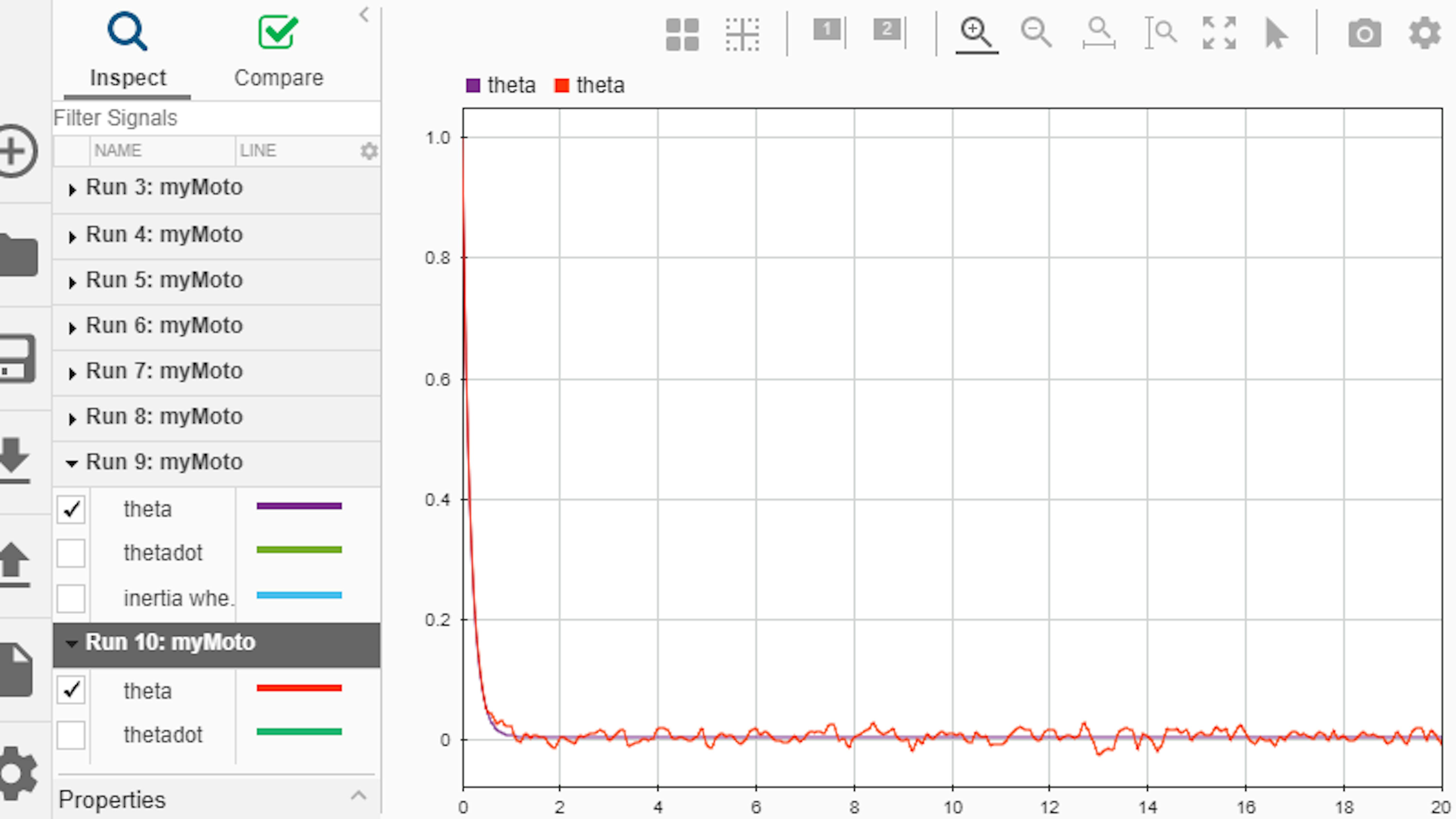
According to the data obtained from the simulation (which might look slightly different from the one you see in the image), how do you think your controller performs when facing random environmental perturbations? You can try changing the Kp and Kd values to see whether you can compensate for the error. A typical iterative tuning process would involve testing different noise levels and continuing to tune the proportional and derivative gains to optimize stability, reaction speed, and steady state accuracy.
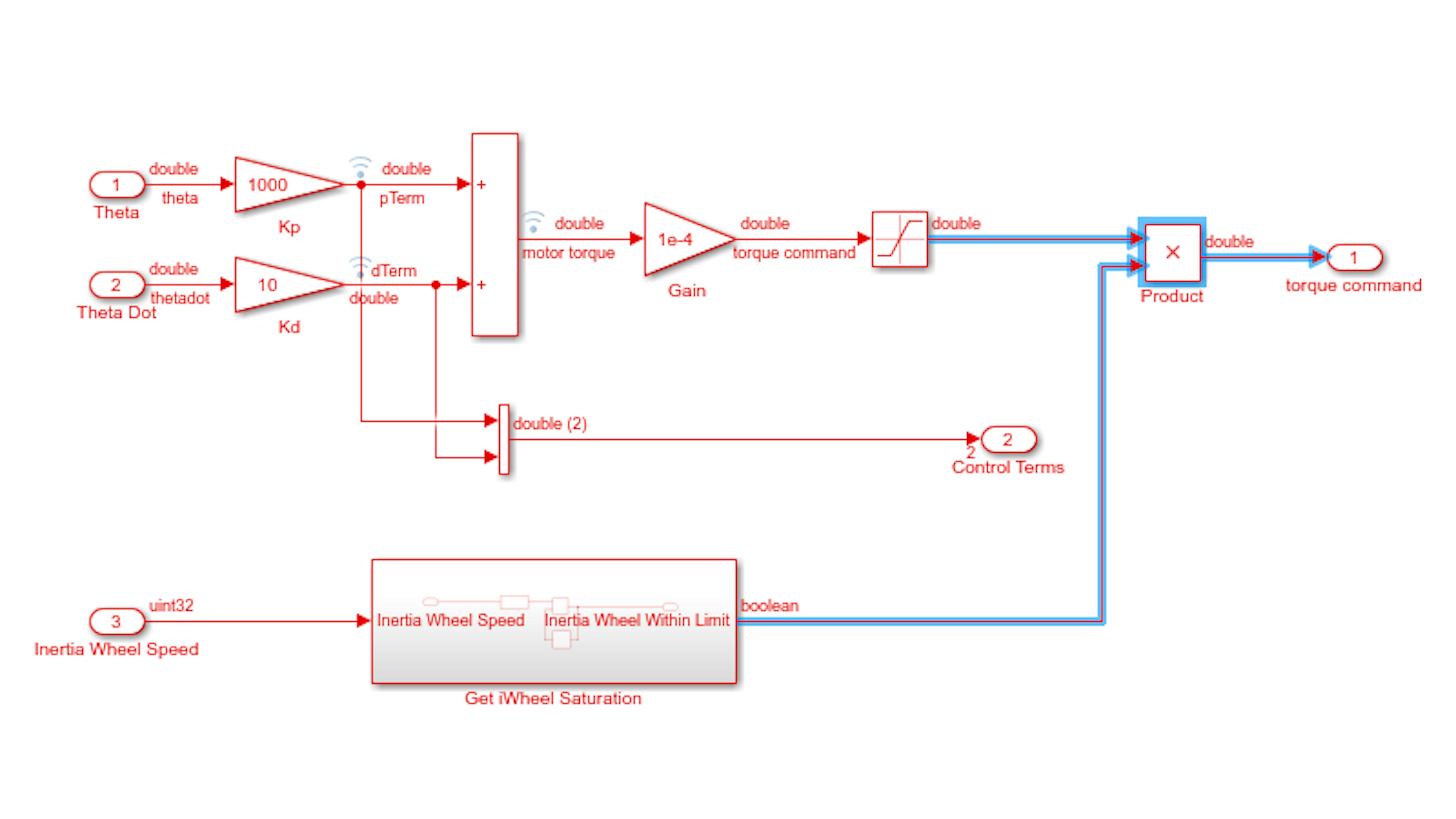
Changing the values empirically will have given you an idea of which control terms are doing most of the work to stabilize the motorcycle. This can be understood much better by looking at some of the signals in the PD controller. Inside the Controller subsystem, label the signals as shown:
Next, select all the signals surrounding the final Add block. Right click on one of the signal lines and select Log Selected Signals from the drop-down list:

Run the simulation and examine the control terms in the SDI view:
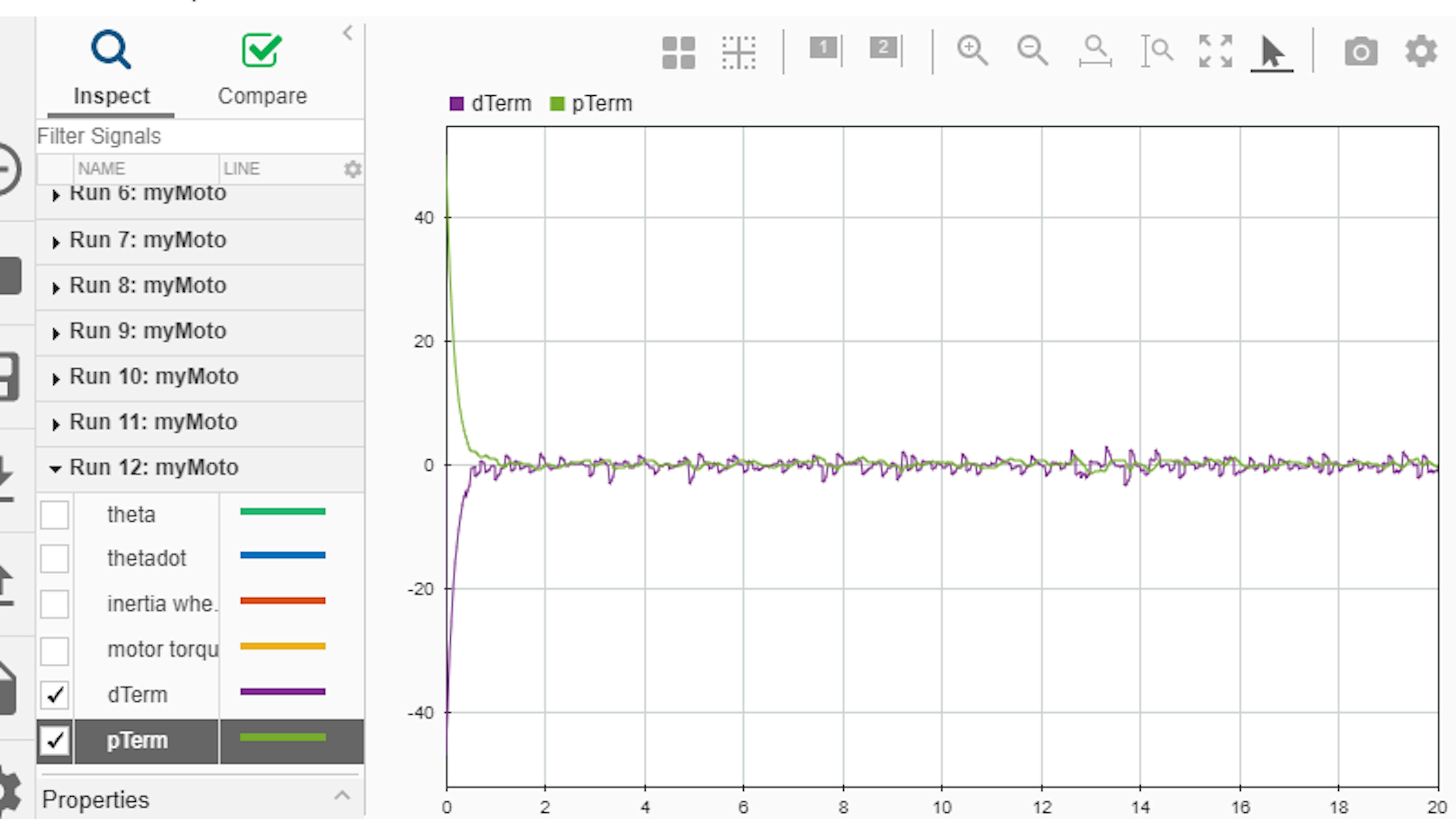
Which term is contributing most of the motor torque?
In this case, they are both providing comparable effort because of the initial non-zero lean angle.
Note: you have done a lot of work with this model, adding modifications to it and so on; please remember to save your system model.
FILES
motoSys0_start.slxmotoSys1_controller.slxEquivalent to myMoto at the end of this exercise.
LEARN BY DOING
You have now learned how to implement a PD controller that will take the lean angle of the motorcycle as parameter, together with the variation of the angle over time. Thanks to these, parameters it is possible to create a Simulink model that will control the inertia wheel’s speed, which will, in turn, help balance the motorcycle.
Furthermore, you have seen how the PD controller responds to different random stimuli and which factors (Kp and Kd) matter the most to counter the undesired torque on the motorcycle that could make it fall. You have also learned how to implement a simulation of a 3D model that responds to behaviors determined by Simulink blocks, something that you will learn how to apply to a real physical motorcycle in later sections in this chapter.
As of now, you are simulating the motorcycle and PD controller while adding a normal distribution of external torque noise to the system. To learn more about the physical behavior of the PD balance control algorithm, try adding other types of disturbance to the system such as a constant, sine wave, or combination of waveforms. Use SDI to monitor what happens to the inertia wheel speed, the motor torque command, the lean angle, and the PD terms. If the behavior is unstable, determine whether you can adjust the PD terms to compensate and restore balance.
EXERCISE 2:
6.2 Program motorcycle components
In this exercise, you will create Simulink models that can control the hardware components of the motorcycle. You will also add custom algorithms (e.g., your self-made PD controller) to these models that can be deployed onto your Arduino directly from Simulink.
You will focus on just a few components: the DC motor controlling the inertia wheel, the tachometer sensor, and the Inertial Measurement Unit (IMU). However, you could apply this knowledge to any components you may want to add to your experiment kit later.
In this exercise, you will learn the following:
- Understand the capabilities and relevant specifications for the inertia wheel DC motor, the tachometer, and the BNO055 IMU.
- Create Simulink models to configure and test individual sensors.
COMPONENTS
Inertia Wheel DC Motor
First, you will set up the DC motor that is used to apply a torque to the inertia wheel, which then causes the motorcycle to exert an equal and opposite counter-torque. Depending on the inertia wheel motor on the kit, use the appropriate hardware specification sheet.
- If your inertia wheel motor has the “12 V DC” sticker you will use this sheet
- If not, you have a 6 V DC motor and you will use this sheet.
Open the iWheel0start.slx model, which looks quite empty as you can see in the following image:
>> iWheel0_start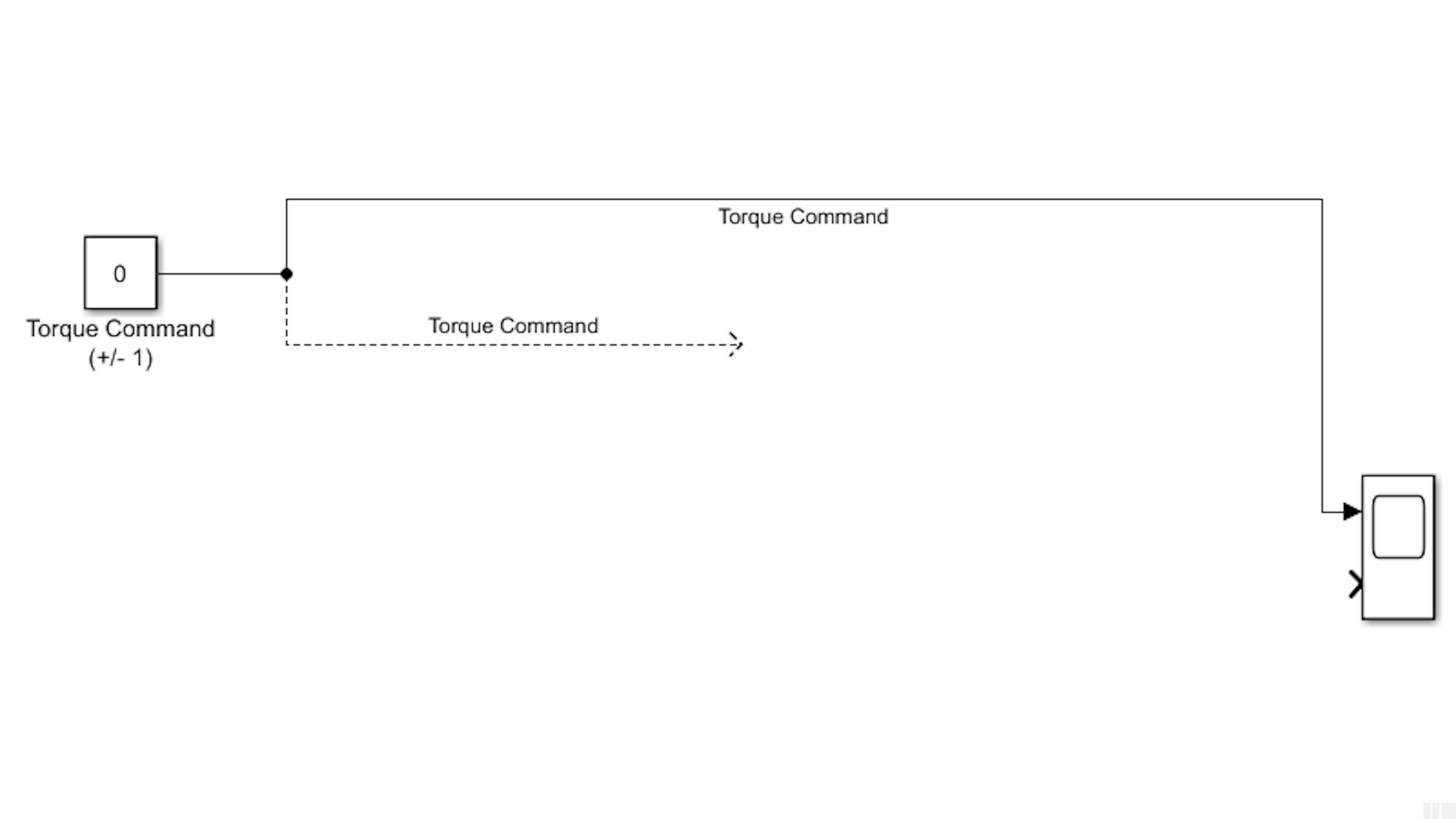
In the following sections, you will be adding blocks to this model to make it accommodate your needs for the realization of the experiments. You will use this model to command torque values to the inertia wheel motor. In your control algorithm, you will determine the necessary motor torque in terms of signed fractional duty cycle (-1 to 1). Later, you will add a tachometer to the model to measure the angular speed of the inertia wheel. Note that in the simulations, we didn’t use the inertia wheel speed as an input to the control algorithm, but this is something that could be handy to make more sophisticated controllers.
Since we are going to be making modifications to the file, give the model a new name; save it as myIWheel.slx.
In the Simulink Library Browser, navigate to Simulink Support for Arduino MKR Motor Carrier, and locate the M3M4DCMotors block:
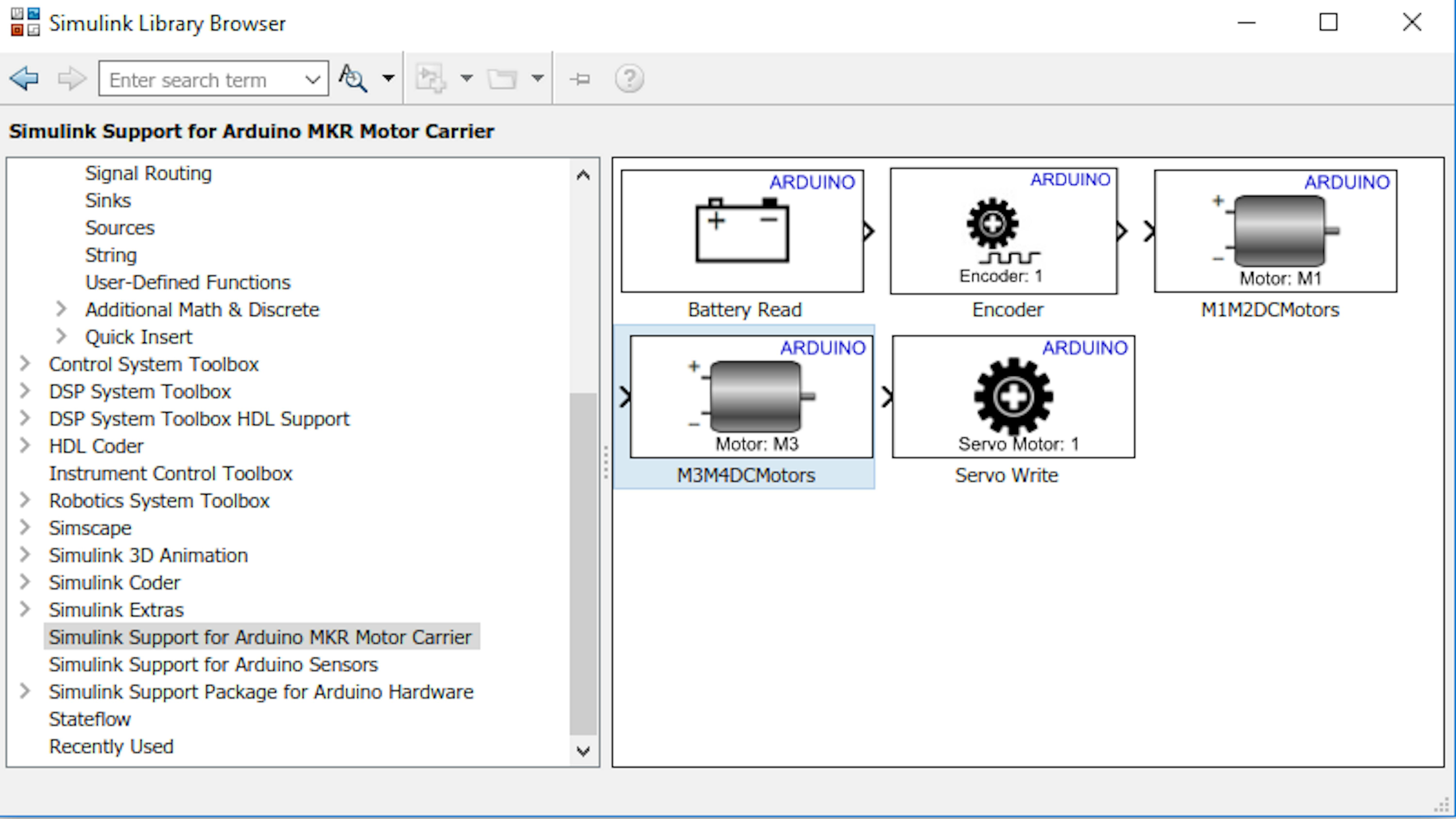
Drag the M3M4DCMotors block into myIWheel.slx:
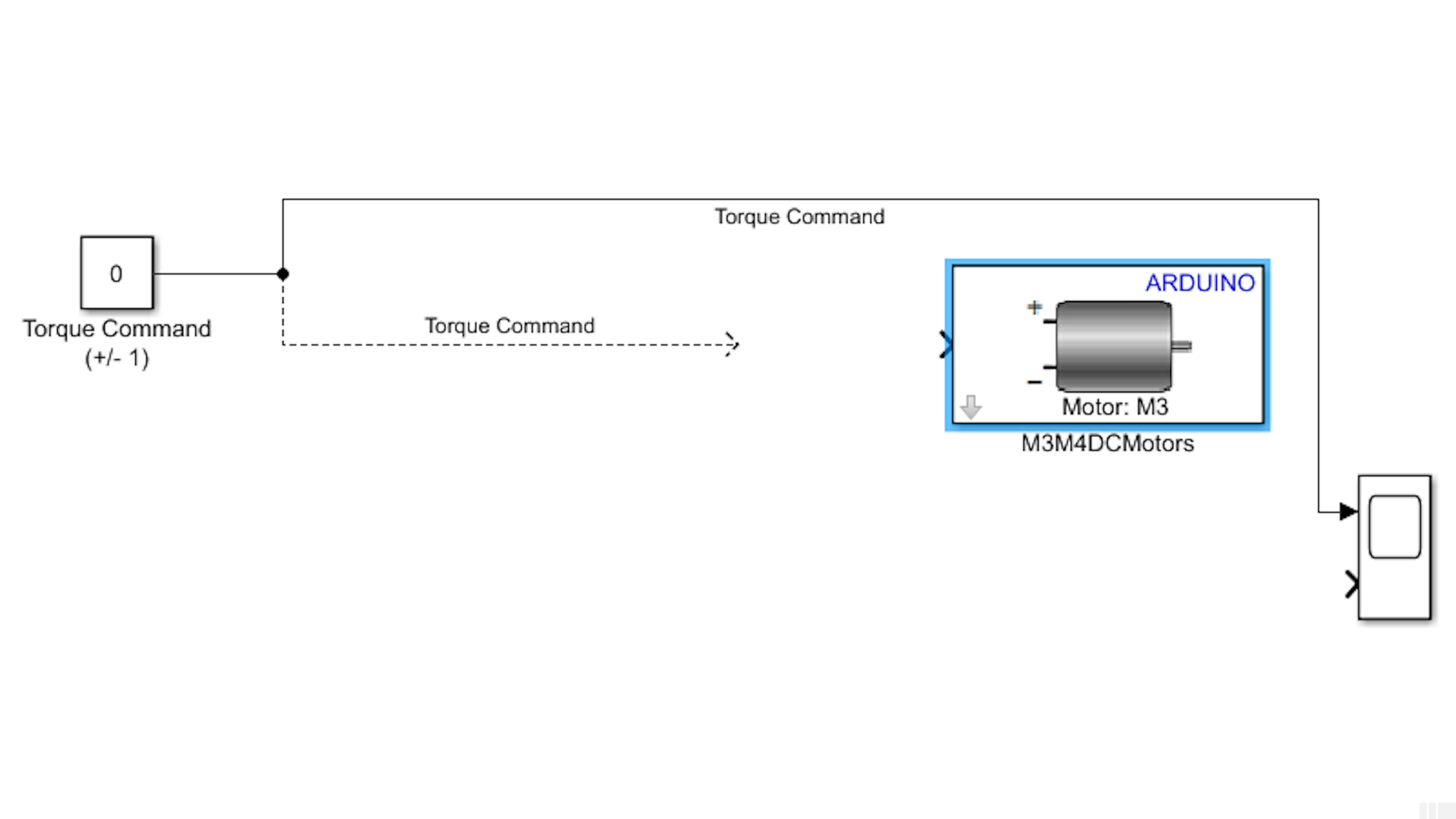
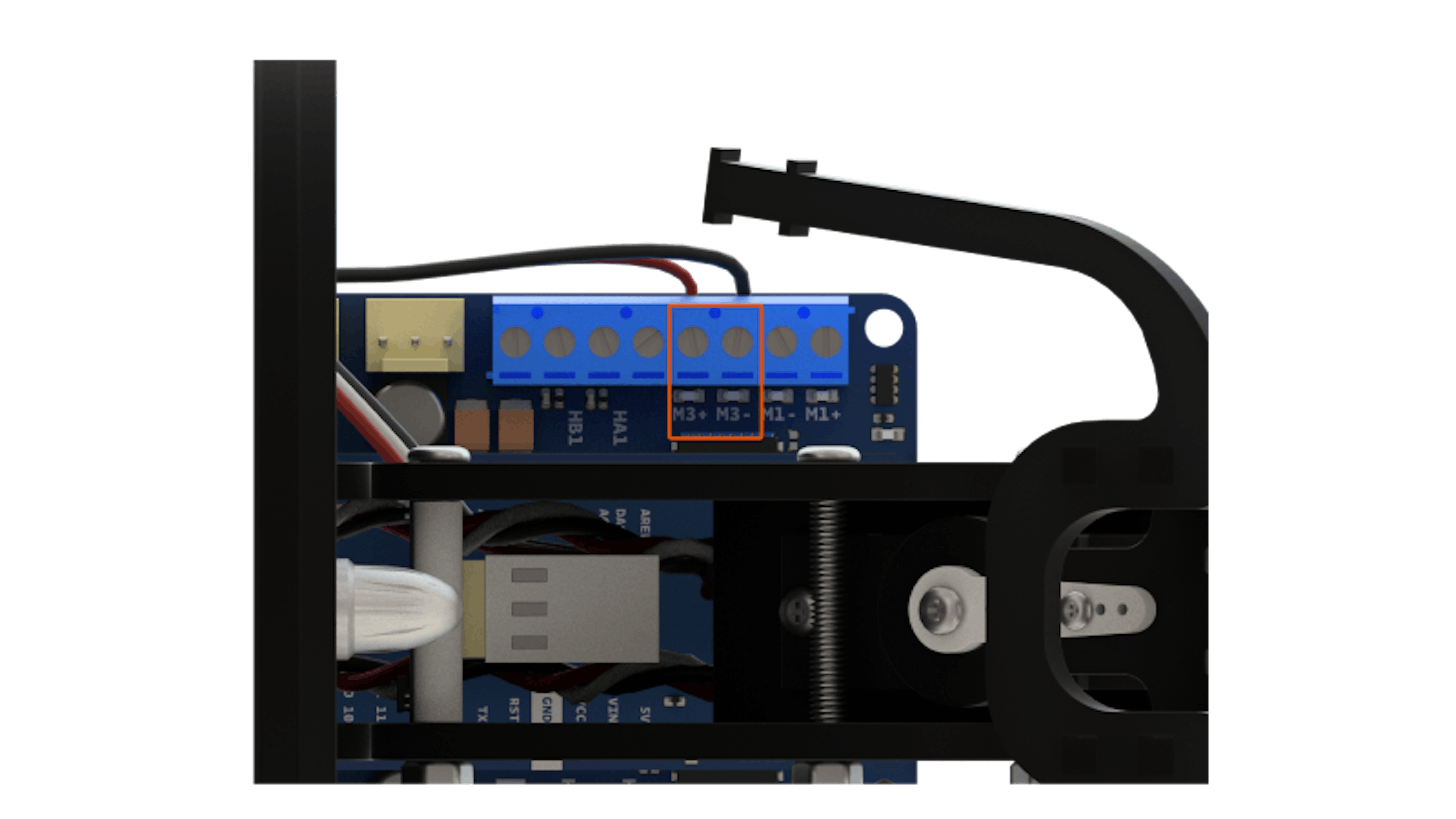
Check the wiring of your inertia wheel motor and see where it is connected to the motor carrier. You will need this information in the next step.
Open the DC Motor block dialog and set the Motor port drop-down accordingly:
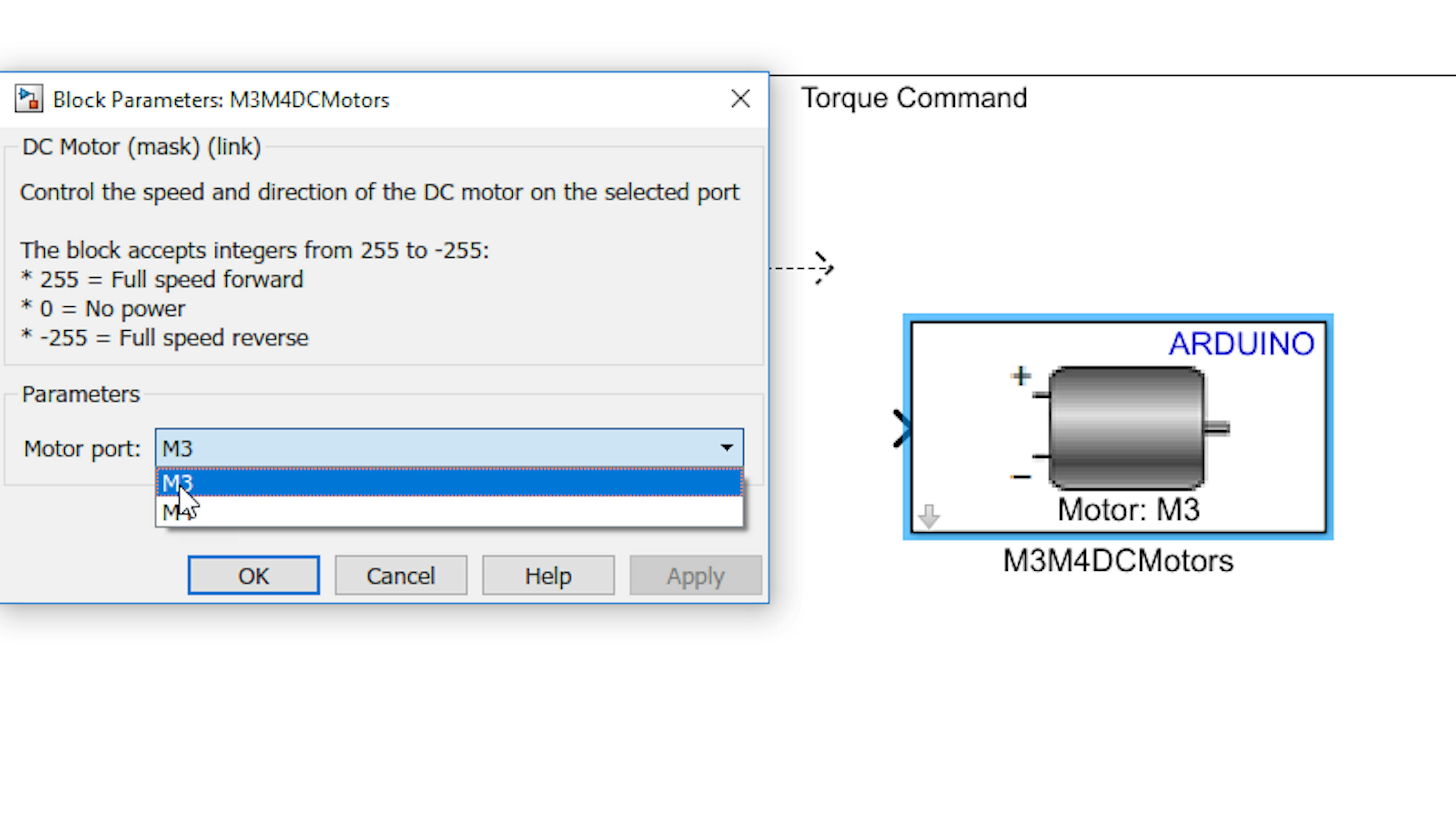
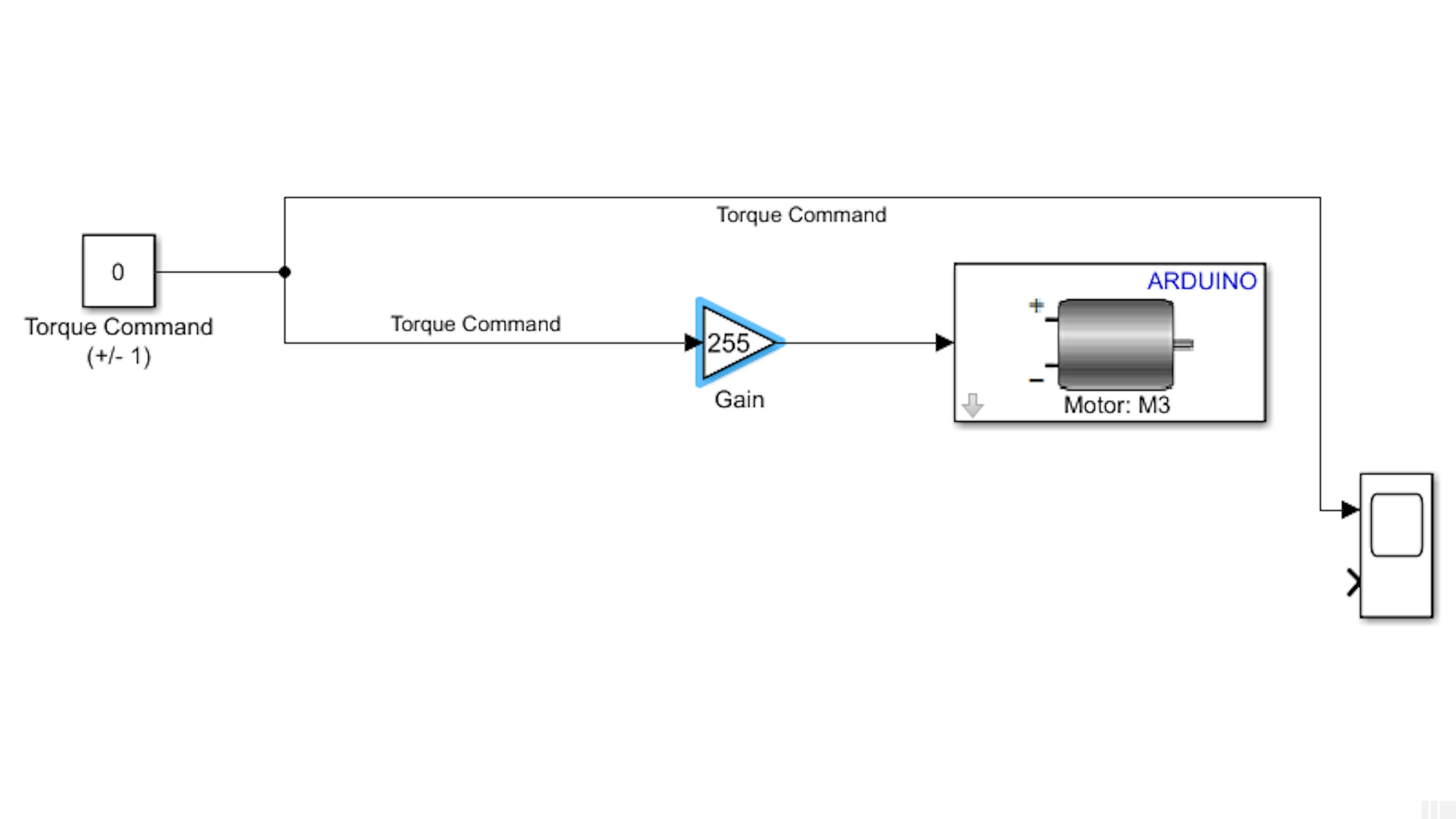
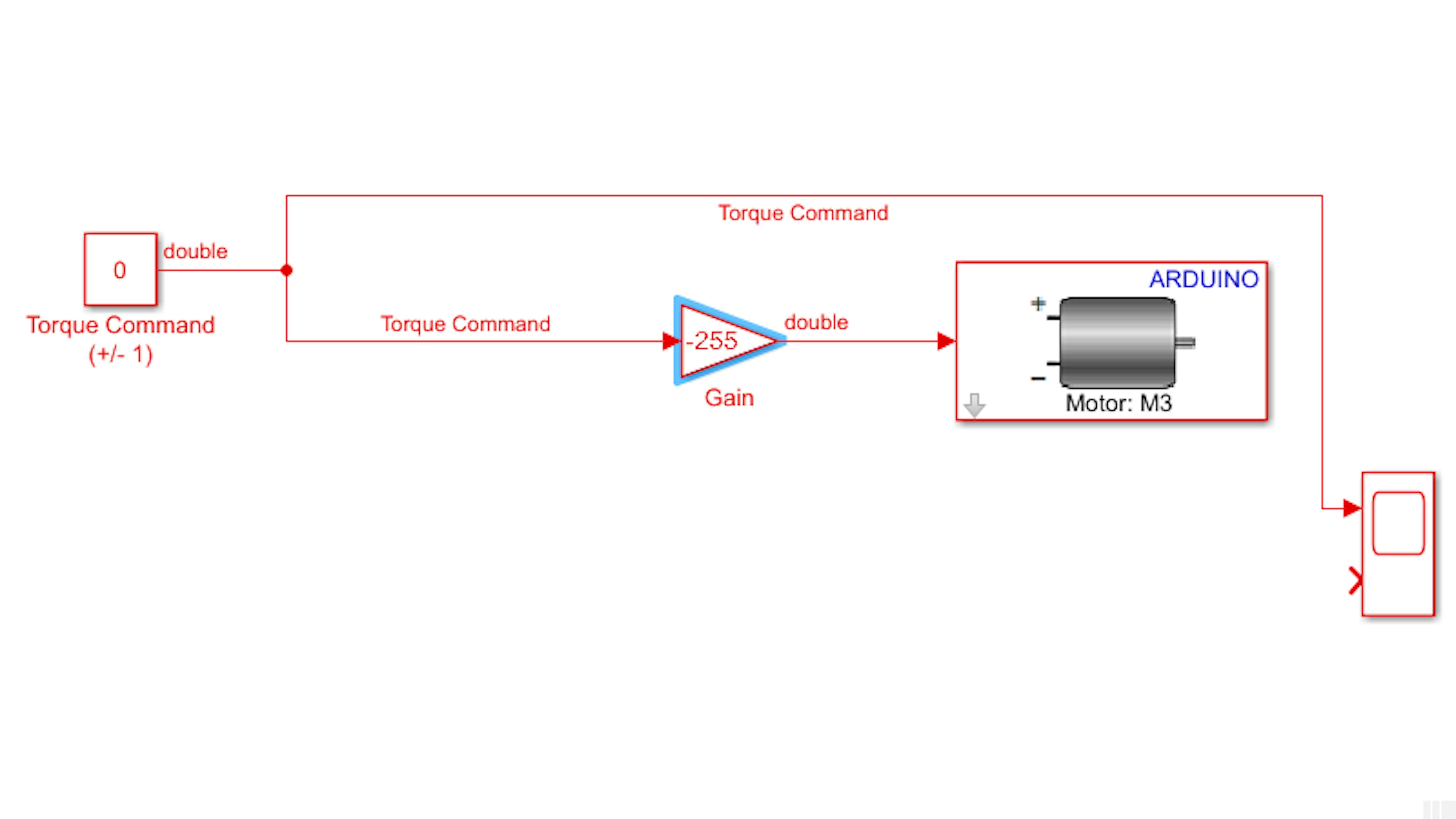
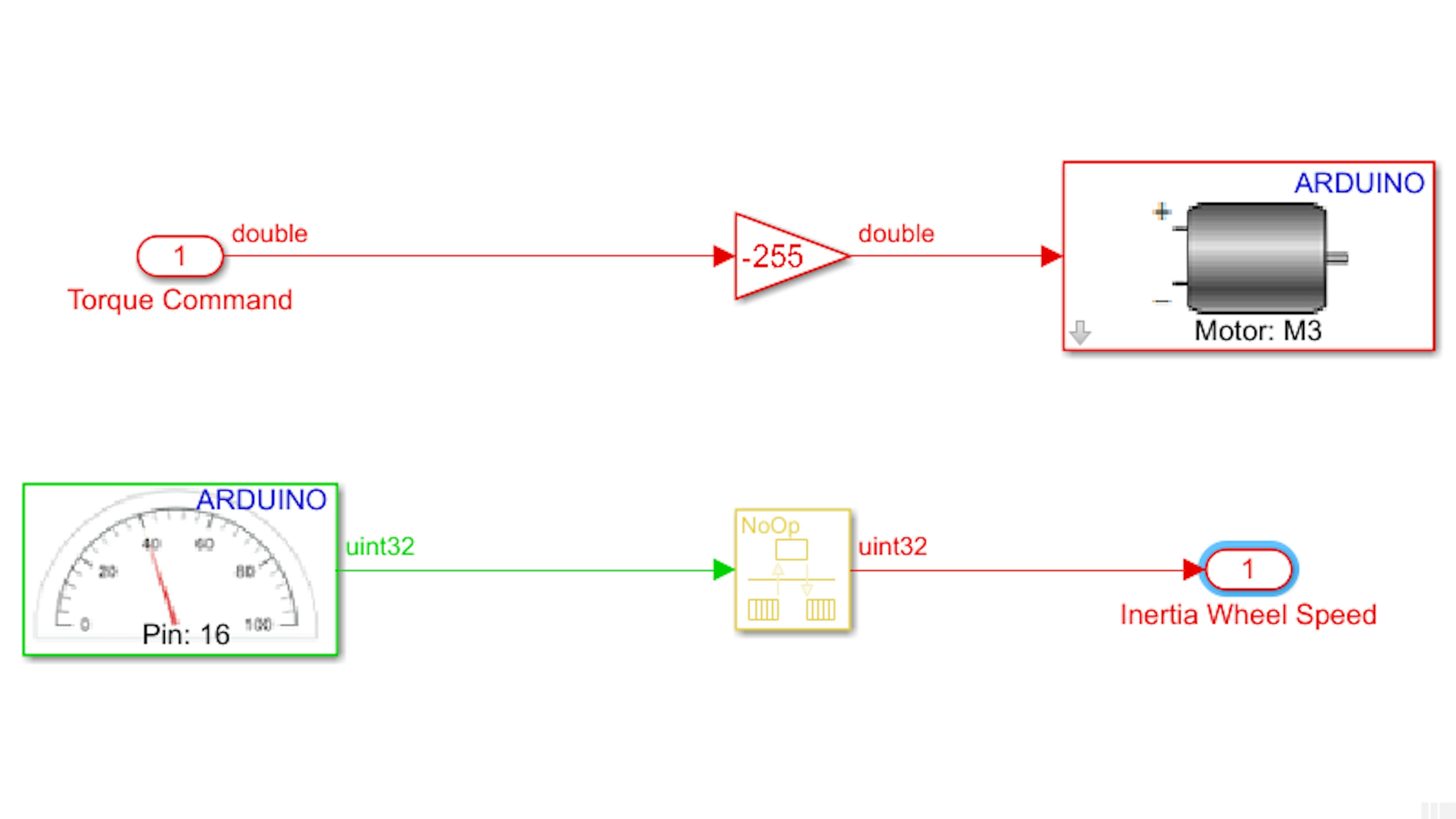
The M3M4DCMotors block has one input that indicates both the voltage to be applied across the motor leads and the direction in which to apply it. A positive input between 0 and 255 indicates that a positive torque should be applied to the motor, while a negative input from -255 to 0 indicates a negative torque. The input value gets normalized, rounded, and transmitted to the appropriate PWM channel for positive or negative motor torque as an 8-bit unsigned integer between 0 and 255. The controller that we saw in the previous chapter generated a motor torque command between -1 and 1. To get the torque command into the proper format for the DC Motor block, go to the Simulink Library Browser and add a Gain block from Simulink → Math Operations. Set the gain value to 255 and connect the blocks as shown:
Now you are ready to run the model on the motorcycle. To do that, first you will need to connect the USB cable between your computer and the MKR1000. Then power on the MKR Motor carrier using external battery and then press the Run button from the toolstrip in your Simulink model. Experiment with different torque commands between -0.5 and 0.5.
Note: Be careful not to let the inertia wheel spin too fast or for too long, as it may overheat the motor or cause structural damage to the motorcycle. You will learn later how to mitigate this risk using the tachometer block
As you run the model, examine the motorcycle from behind. Pay attention to the direction of angular acceleration when the torque command is positive and negative. If your wiring is same as the instructions video, then when the torque command is positive the inertia wheel will accelerate clockwise. If it spun counterclockwise, interchange the wires connected to M3+ and M3-. For modeling consistency later, you want to make sure that the torque command and the lean angle θ are defined with the same polarity. This means that when viewed from behind, θ should increase counterclockwise, and a positive torque command should drive the inertia wheel counterclockwise. Change the gain value to -255:
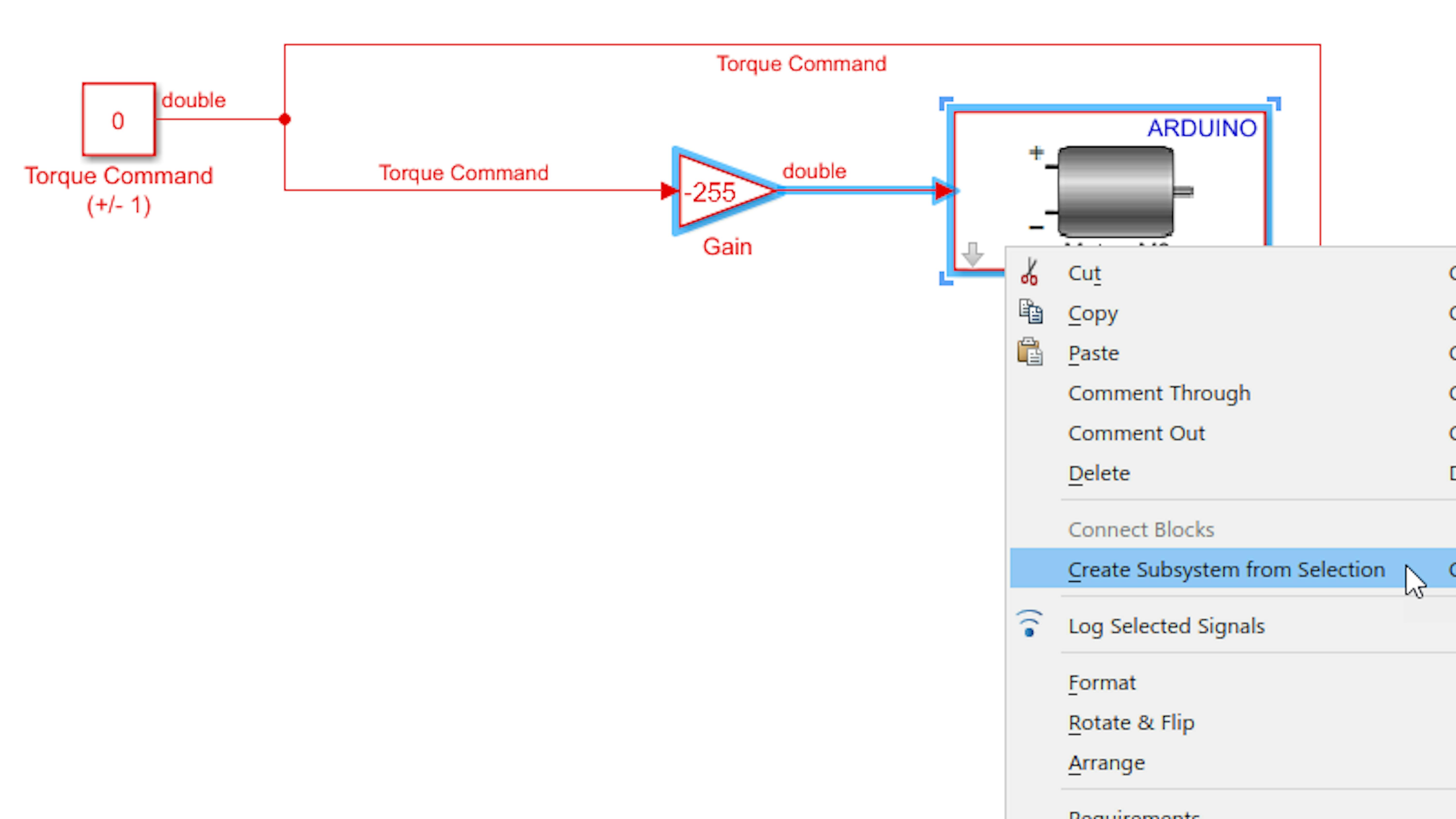
Finally, let’s clean things up by making a subsystem. Select the Gain block and the M3M4DCMotors block, right-click, and select Create Subsystem from Selection:
Label the new subsystem Inertia Wheel. You will end up with something similar to what is displayed in the next figure:
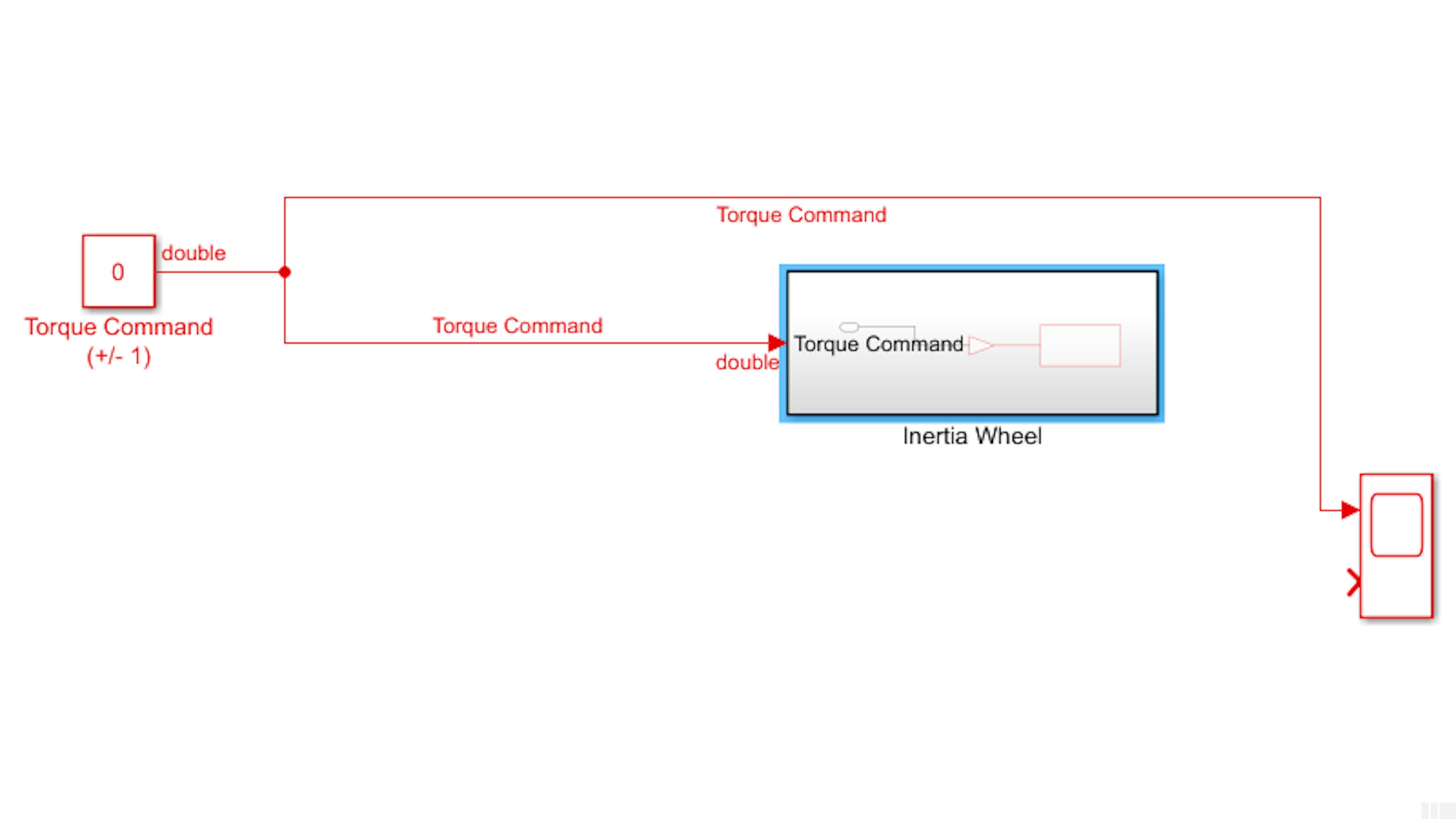
Run the model once more to confirm the correct behavior.
Tachometer
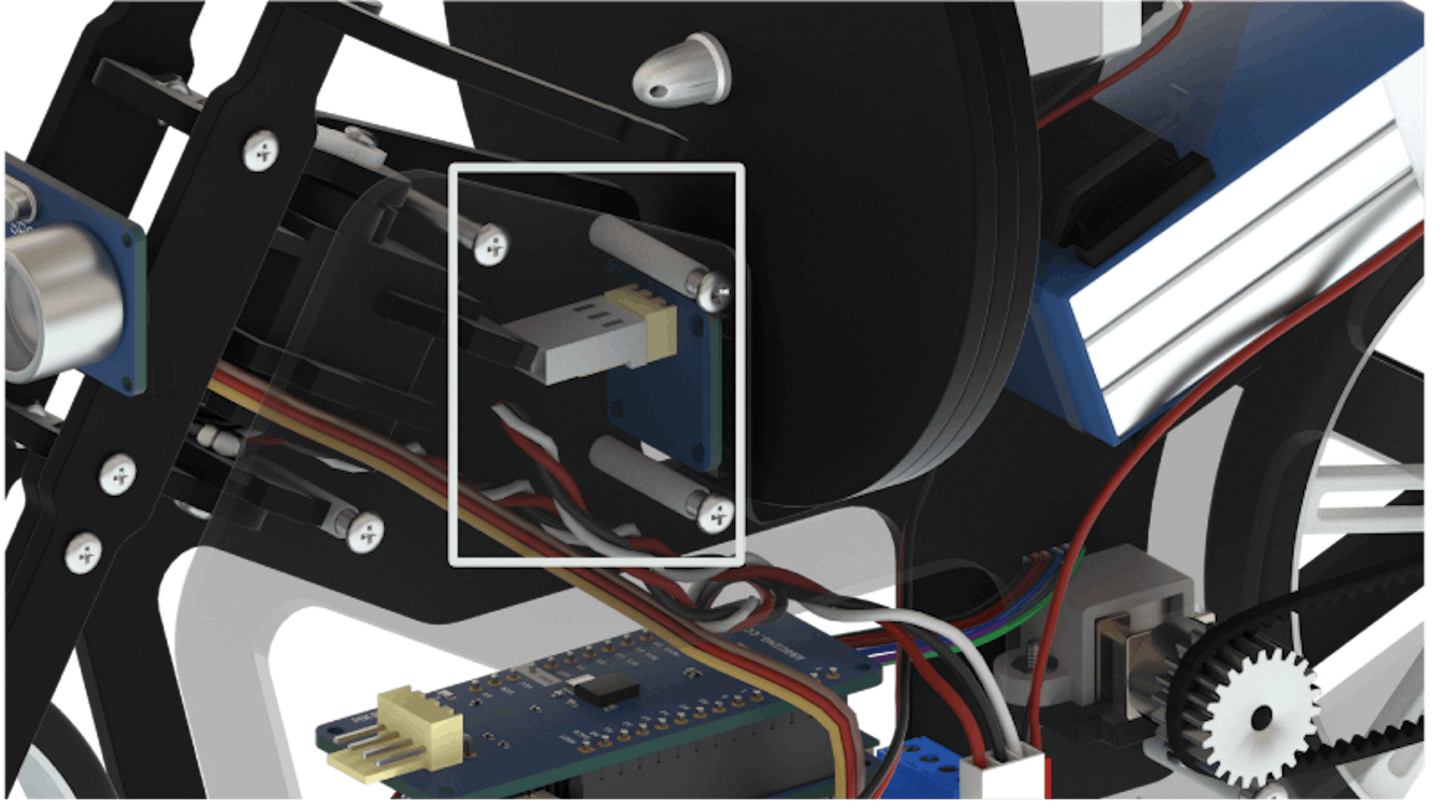
The inertia wheel DC motor can spin extremely fast when full torque is applied for a sufficient duration. However, spinning the inertia wheel too fast for too long can permanently damage many components of the motorcycle, including the DC motor (overheating and melting), the motor carrier (overcurrent damage and overheating), and the structural members (vibrational stress and heat distortion). You want to be able to spin the inertia wheel fast enough to keep the motorcycle balanced but not so fast that you end up damaging it. To mitigate this risk, the motorcycle includes a tachometer inside the plastic casing directly in front of the inertia wheel:
Review the hardware specs for the SL353 series micropower omnipolar digital Hall-effect sensor (tachometer) included in the kit. The sensor contains an electromagnet that is connected to a digital circuit which holds a value of 1 when an external magnetic field of a certain magnitude is applied and 0 when it is not. During the assembly, you added two magnets 180 degrees apart that effectively exert magnetic field pulses on the tachometer when the inertia wheel rotates:
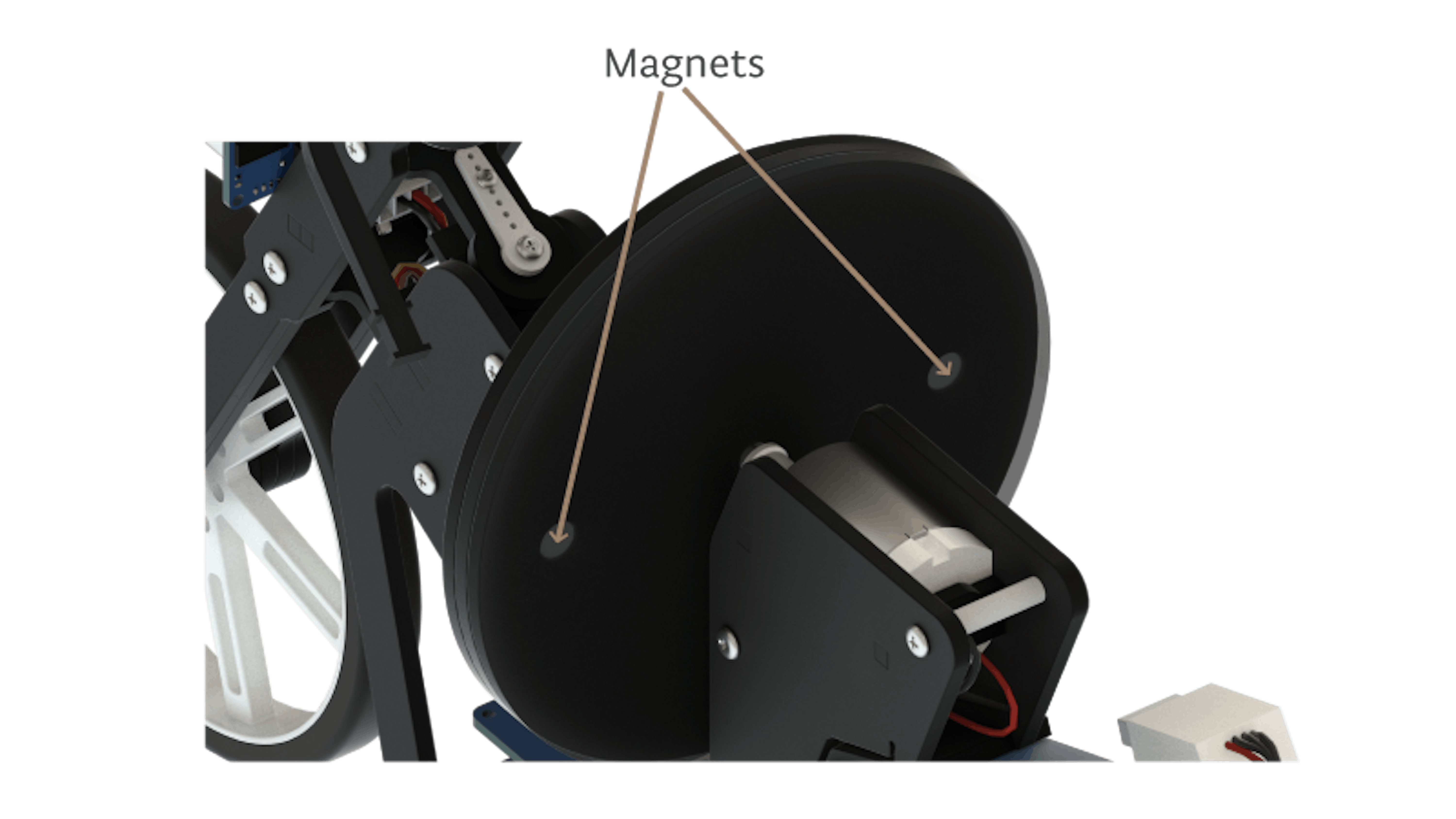
The Hall-effect sensor’s digital circuit contains logic to keep track of how many magnetic field pulses have taken place since power was last reset. You can use this information to determine the approximate angular speed of the inertia wheel over some time interval. You can then set a threshold for the angular speed such that the inertia wheel motor shuts off and remains off when the limit is first exceeded. You should then leave the hardware alone for a few minutes to cool off and then restart the application.
To set up the tachometer, open the model myIWheel.slx you were working with earlier:
>> myIWheelNote: If myIWheel.slx is incomplete or unavailable, open iWheel1_test.slx instead and save it as myIWheel.slx.
In the Simulink Library Browser, navigate to the Simulink Support for Arduino Sensors library, and add the Tachometer block inside the Inertia Wheel subsystem in myIWheel.slx, and configure the block as shown:
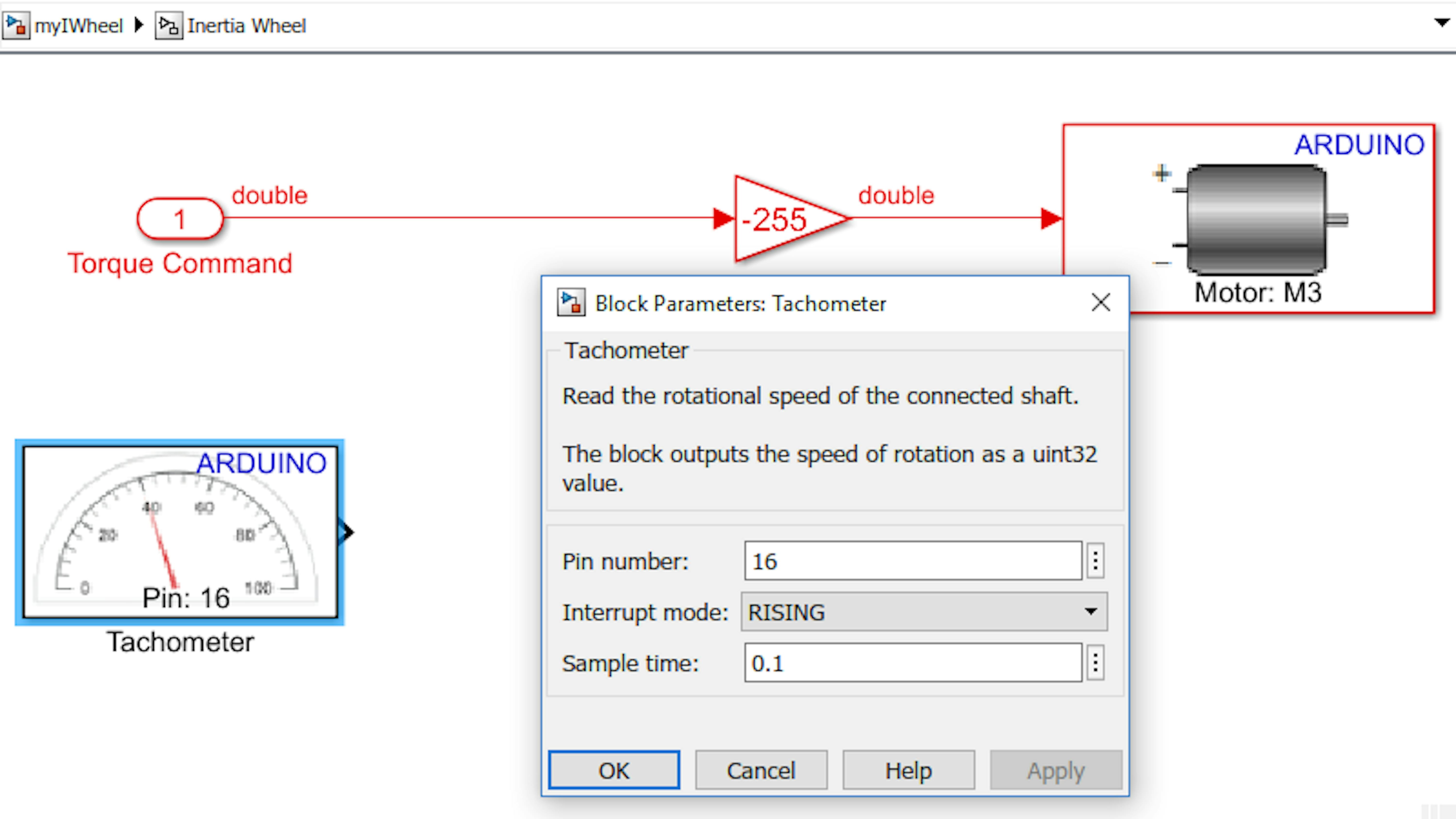
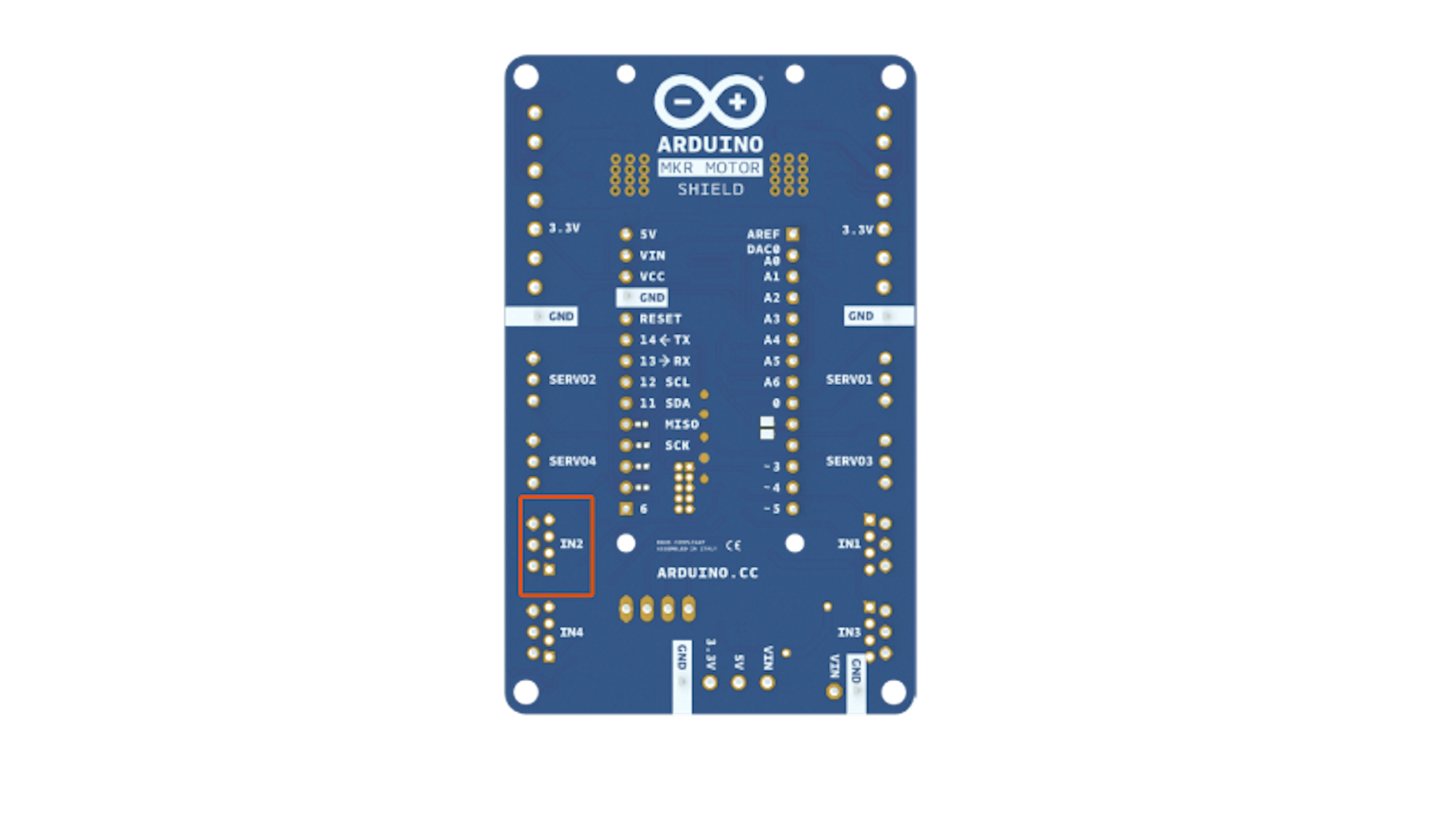
Following the assembly video, you must have connected the Hall effect sensor to Header IN2 on the motor carrier. Examine your motor carrier and locate the Hall effect sensor connection and make sure it is connected to port labelled IN2. The Pin number property here indicates the low-level pin that is being used and 16 is the appropriate number for IN2 connector.
Interruptible pins are needed to update the tachometer count whenever changes in the digital value occur, regardless of the rest of the application’s periodic execution schedule. Interruptible pins on microcontrollers can stop the whole processor to perform a certain callback routine whenever there is a change on the pin. The Interrupt Mode property indicates when to increment the tachometer count, with respect to the waveform of the digital 0 or 1 that indicates whether there is an external magnetic field present. The Interrupt Mode RISING means that the pulse should change from 0 to 1 for the change to trigger the interrupt. The Sample Time property indicates how frequently, in seconds, the count is output from the block and then reset to 0. If the sample time is set too low, you might have periods where no counts occur even though the inertia wheel is spinning. If the sample time is set too high, you may miss changes in the inertia wheel’s angular speed that occur within one period. For this application, we are going to use 0.1 seconds as the sample time, a value we have calculated theoretically — and tested empirically — to be working.
For our purposes, the units of angular speed are irrelevant as long as the speed threshold is expressed in the same units. Thus, we will report the inertia wheel speed in counts per 0.1 second.
Since the tachometer executes at 10 Hz (the period of 0.1 in sampling rate corresponds to 10 Hz, and the rest of the model at 100 Hz (0.01 sampling rate), you will need a Rate Transition block to hold the tachometer output for 10 controller execution cycles. To do this, add a Rate Transition block from Simulink → Signal Attributes:
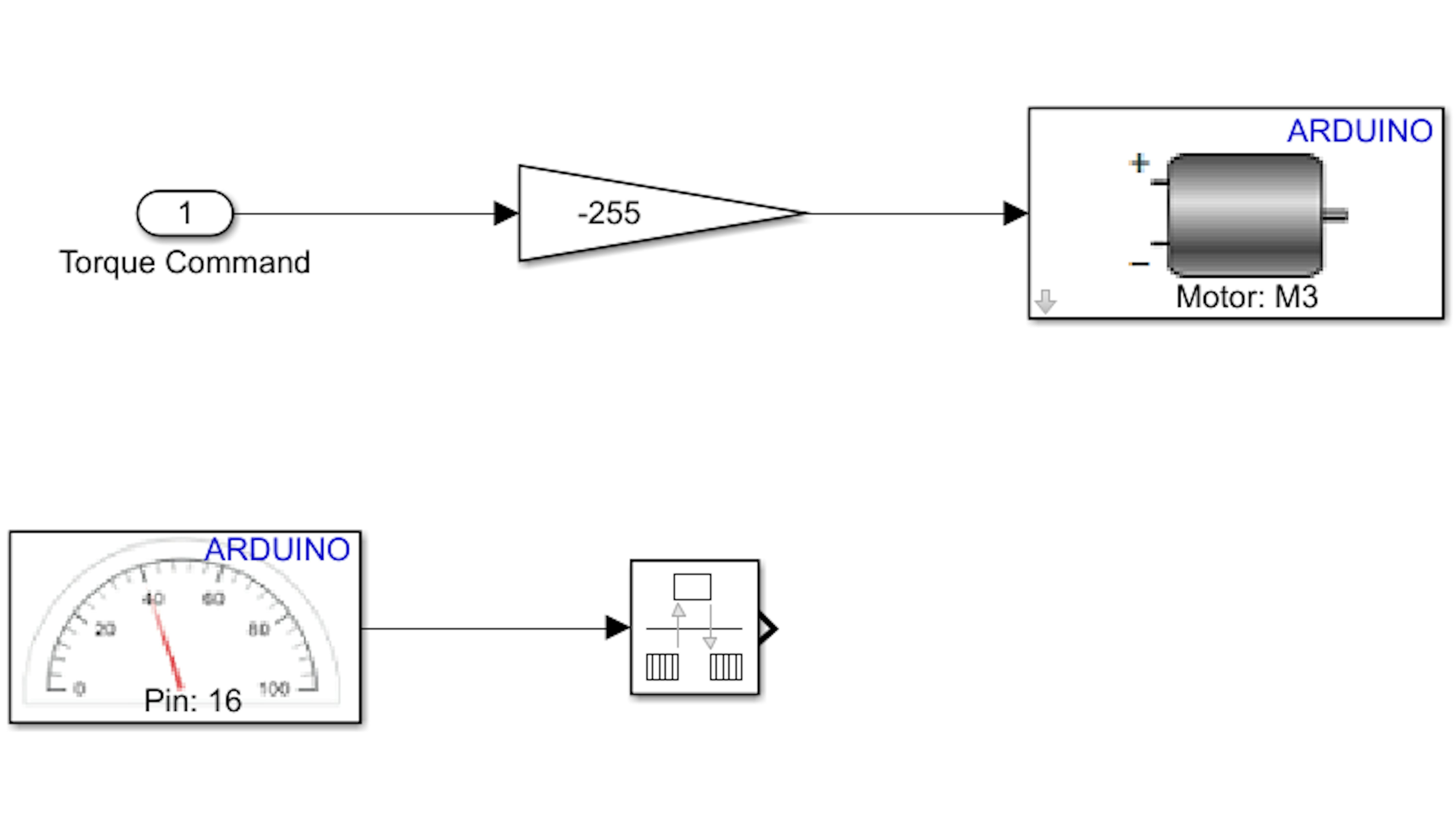
Finally, add an Out1 block from Simulink → Sinks and label it as shown. Press Ctrl + D to see the sample time color coding:
Return to the top level of the model and connect and label the Inertia Wheel Speed signal as shown:
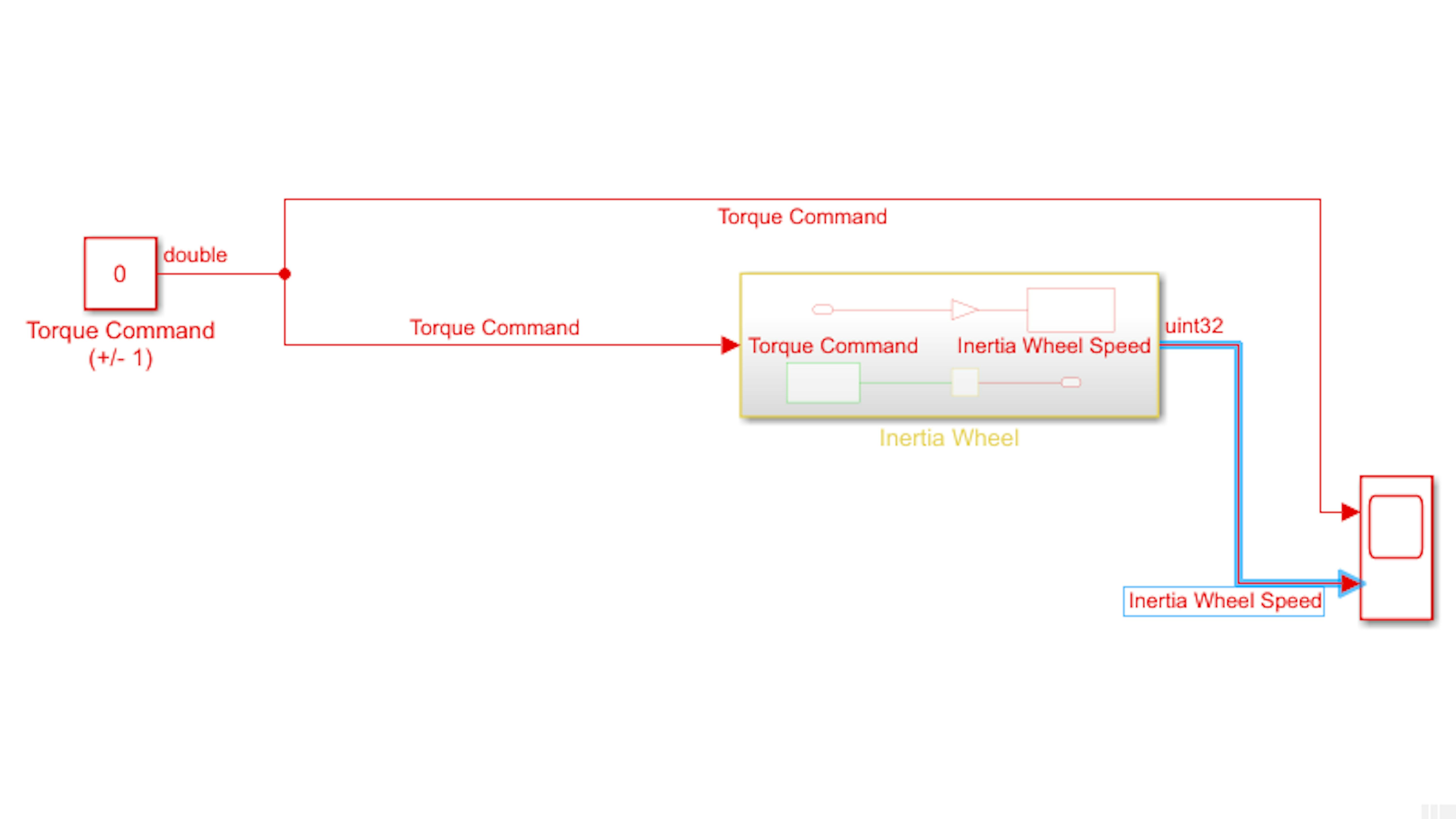
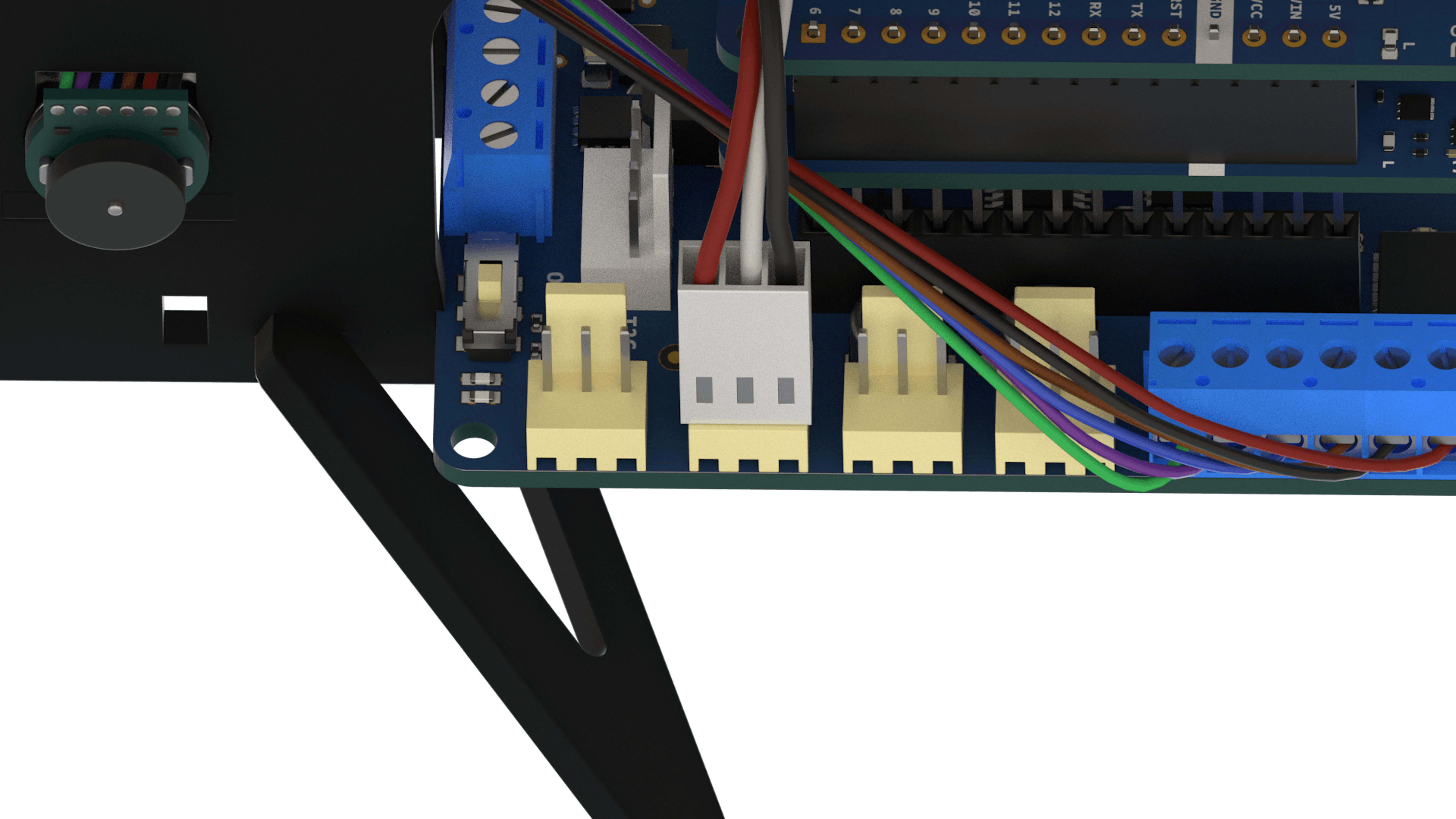
Now, let’s test it out! Locate the three-wire bundle originating from the tachometer circuit and ensure that it is plugged into the IN2 port on the motor carrier:
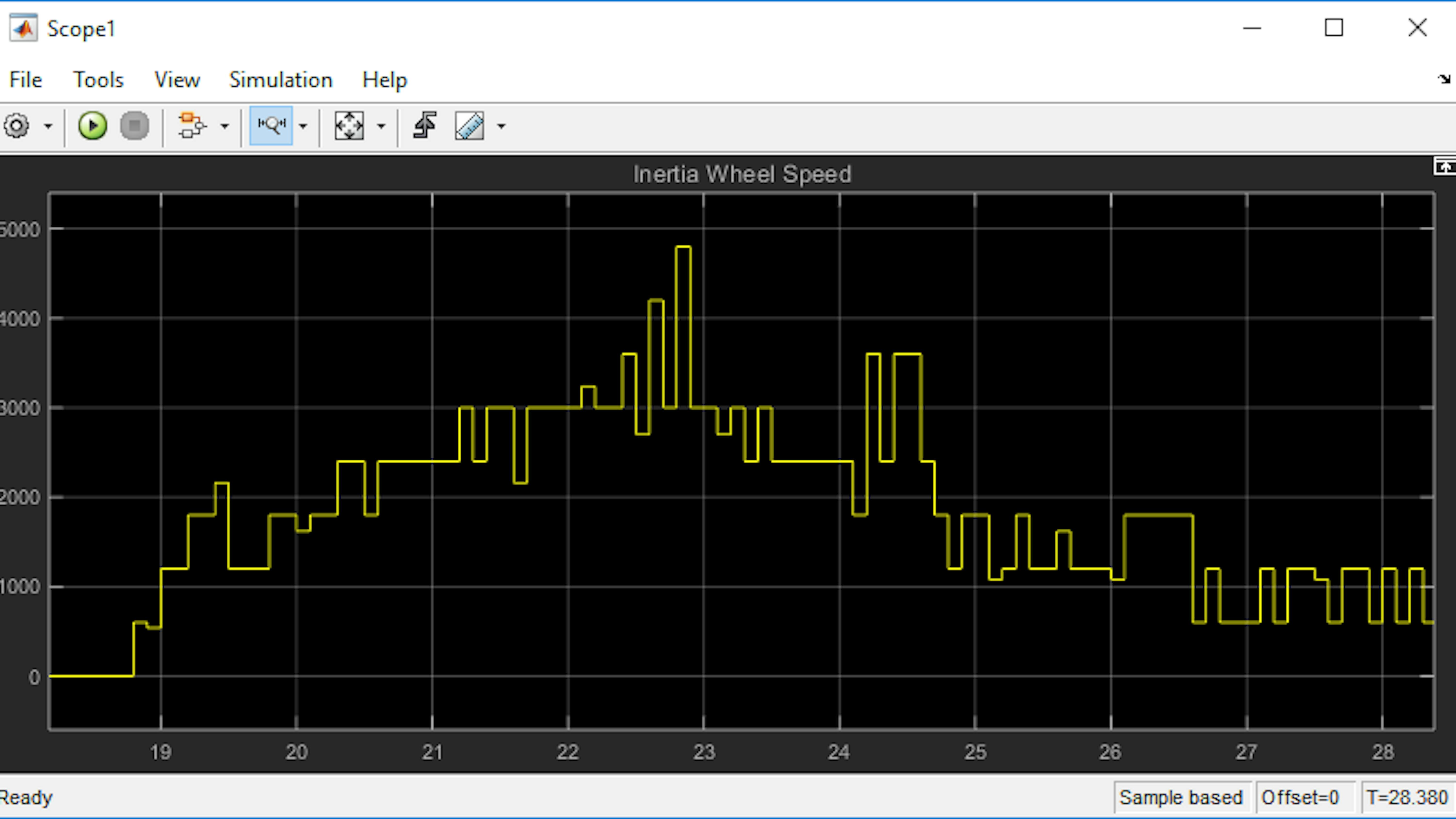
Set the Torque Command constant to 0. Run the model and observe the tachometer output in the Scope block. Try first by manually rotating the inertia wheel without the motor and seeing if any tachometer count shows up. Then try commanding a low torque command to the motor, e.g. 0.2. Pay attention to the behavior of the inertia wheel speed when the torque command is held constant for some time. Do NOT command a large torque value (more than +/- 0.5) for more than a few seconds:
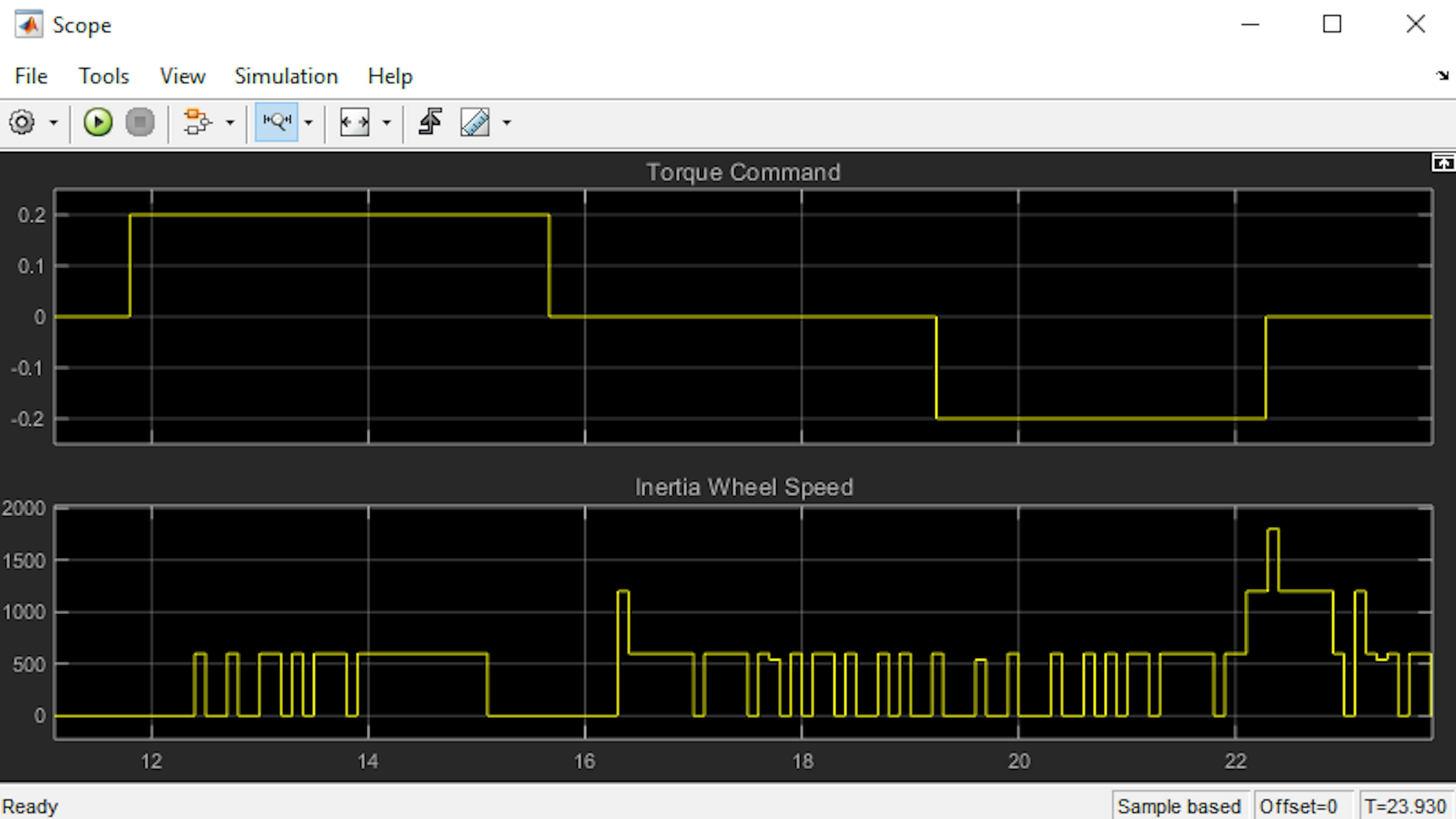
Note: Your plot might look different compared to this as the motors are different.
Why doesn’t the inertia wheel speed increase indefinitely when torque is applied from the motor? The answer is friction. Most restorative forces, including solid-solid friction, have a term that increases with the relative speed of the objects. As the inertia wheel speed increases, the frictional torque in the motor also increases until a terminal angular speed is reached. Here the frictional torque is equal and opposite to the applied motor torque. Thus, you can never reach infinite angular speed. However, when the frictional force is high, lots of heat is generated by the motor and could lead to irreversible damage. Note how this differs from the simulation we made earlier where we assumed zero friction on the wheel.
Does a negative torque command result in a negative inertia wheel speed? No. The tachometer only measures how many times the external magnetic field pulse has been raised and/or lowered. It has no way of knowing which direction the external magnet is passing it. This means that you will need to keep track of this information using software.
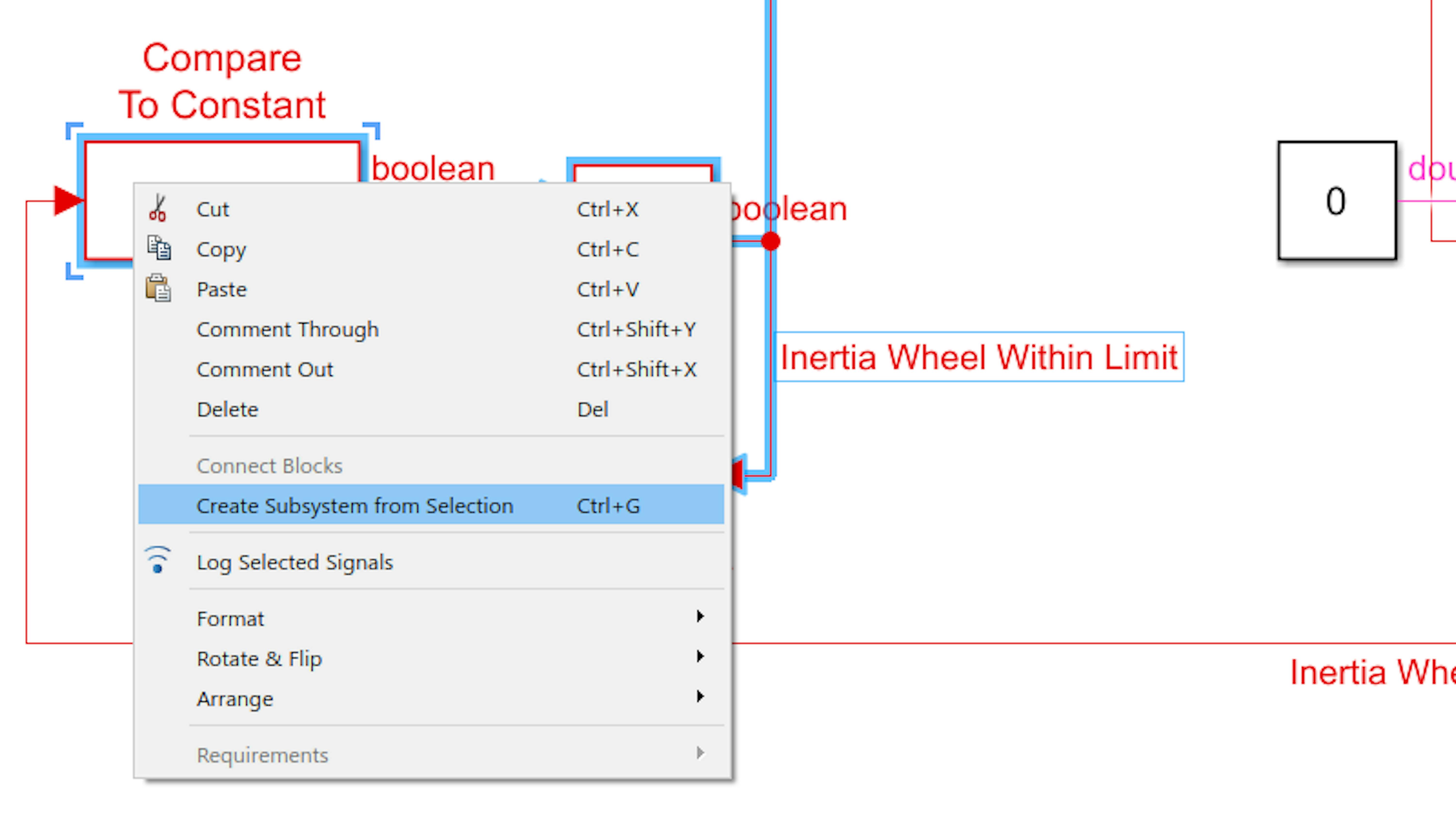
Set the Torque Command constant to 0 and stop the model. Now, we’ll add some logic to turn off the inertia wheel motor when the speed is too high (and keep it off until the application is restarted). Let’s start by comparing the measured inertia wheel speed to a threshold. Add a Compare To Constant block from Simulink → Logic and Bit Operations, and set the operation to <= 4000. Connect the block as shown:
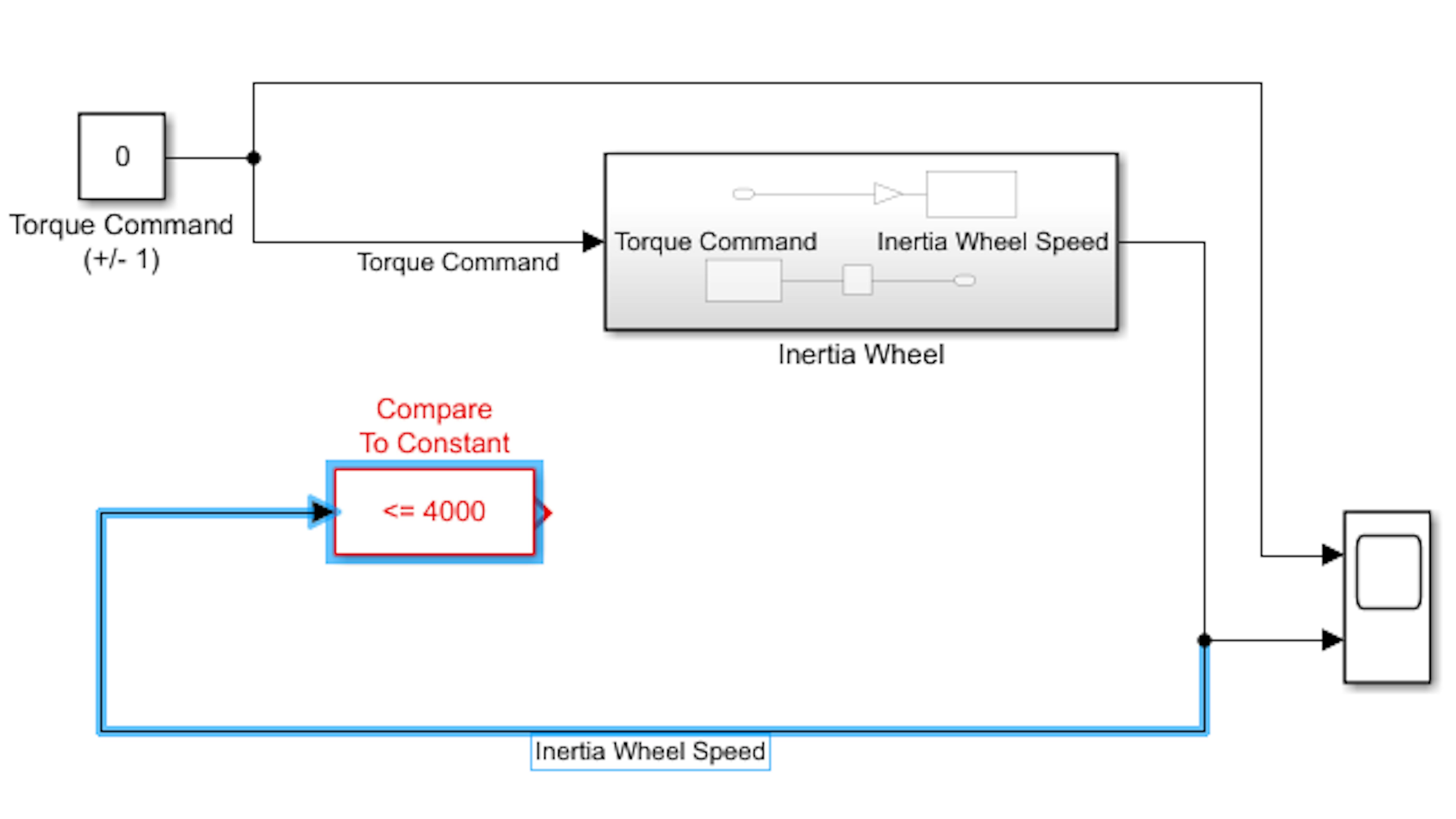
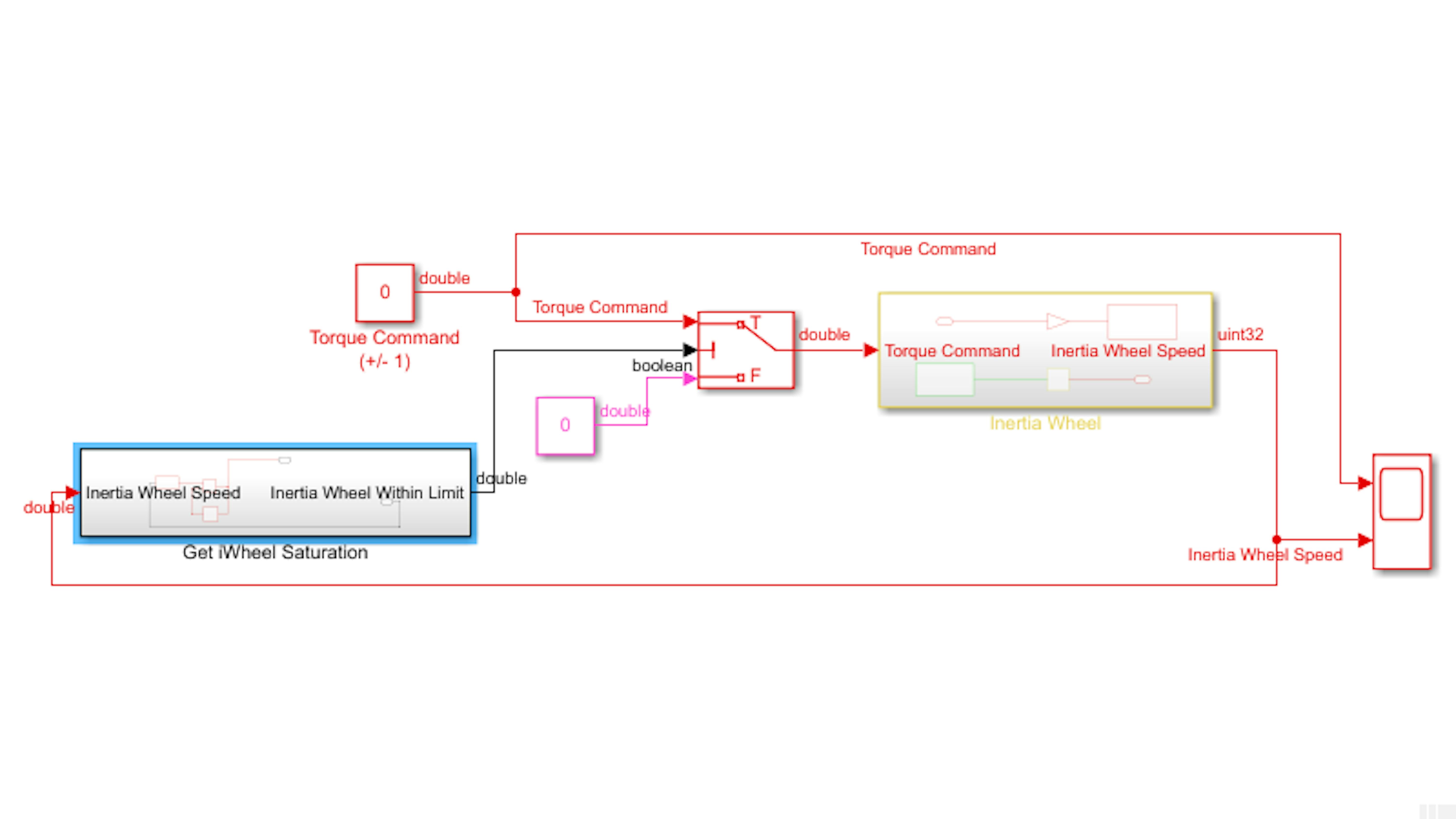
The result of this inequality will determine whether the inertia wheel DC motor is enabled or disabled. Add a Switch block from Simulink → Signal Routing and Constant block from Simulink → Sources. Set the constant value to 0. Reroute the Torque Command signal and connect the blocks as shown:
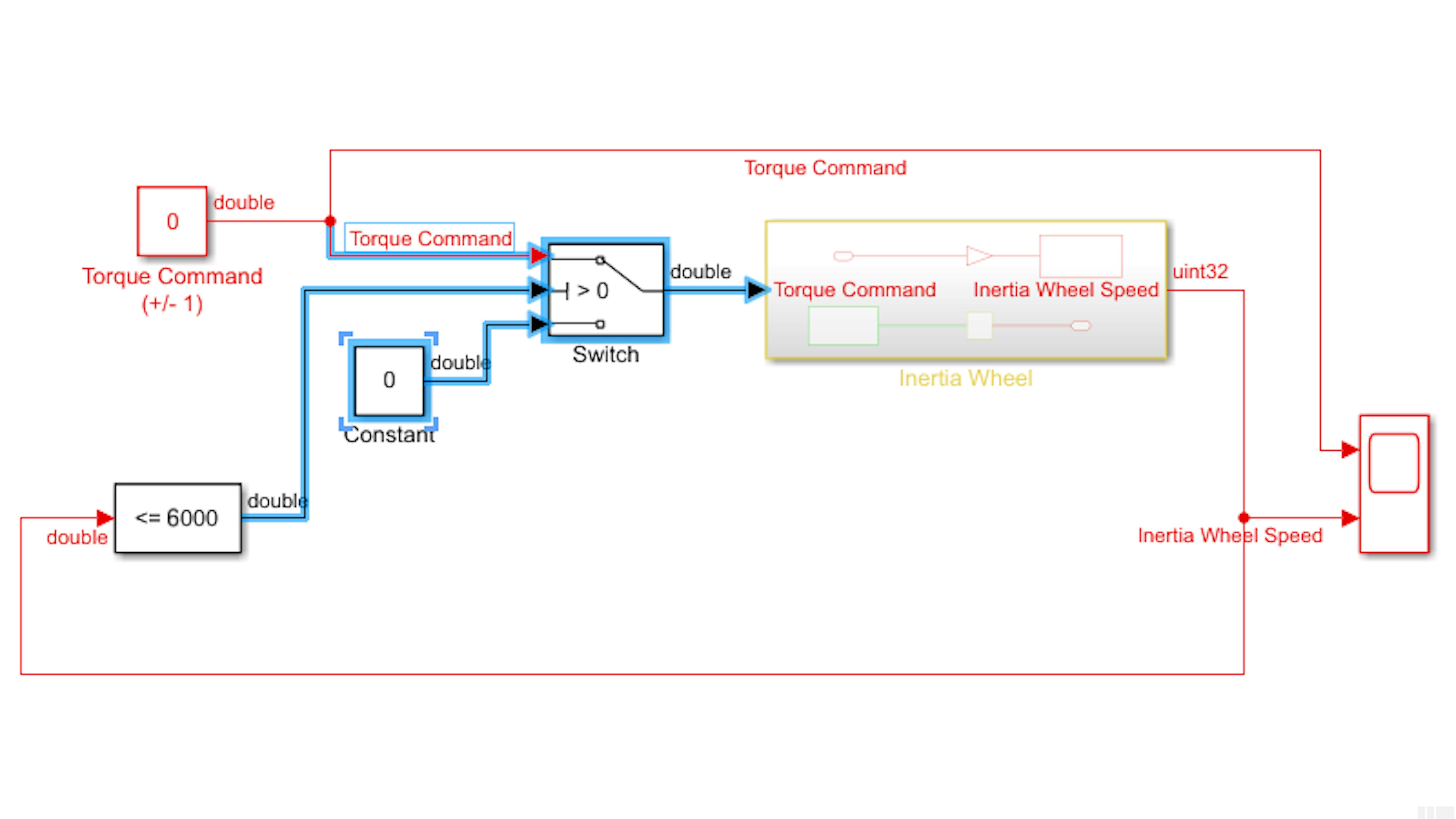
The Switch block will ensure that the user’s torque command will go to the inertia wheel motor if the wheel is not spinning too fast, or a command of zero if the inertia wheel is spinning too fast.
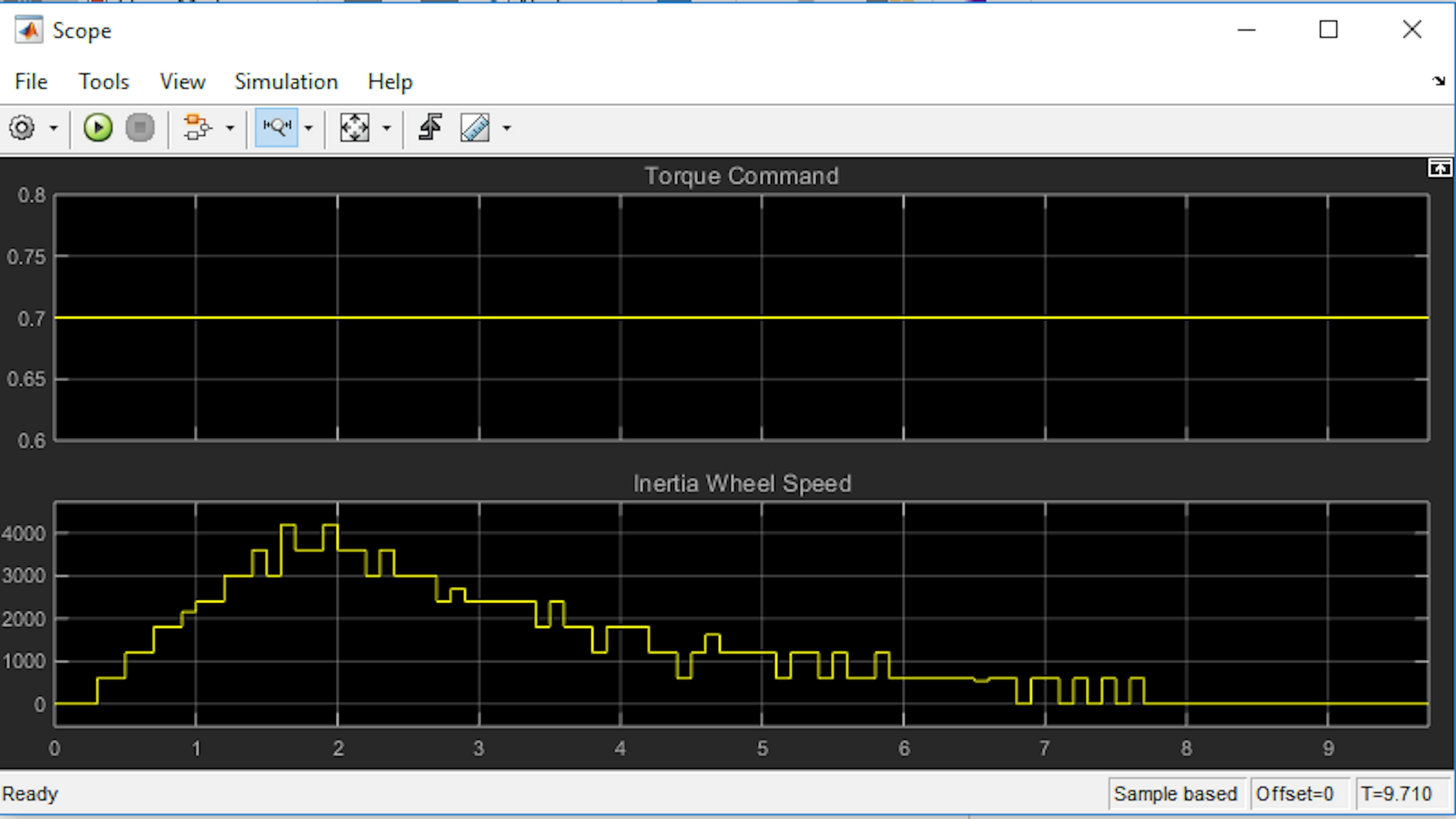
Hold the motorcycle close to vertical position and Run the model. Open the Scope window. Set the torque command to 0.7 and wait for the inertia wheel speed to exceed the threshold of 4000:
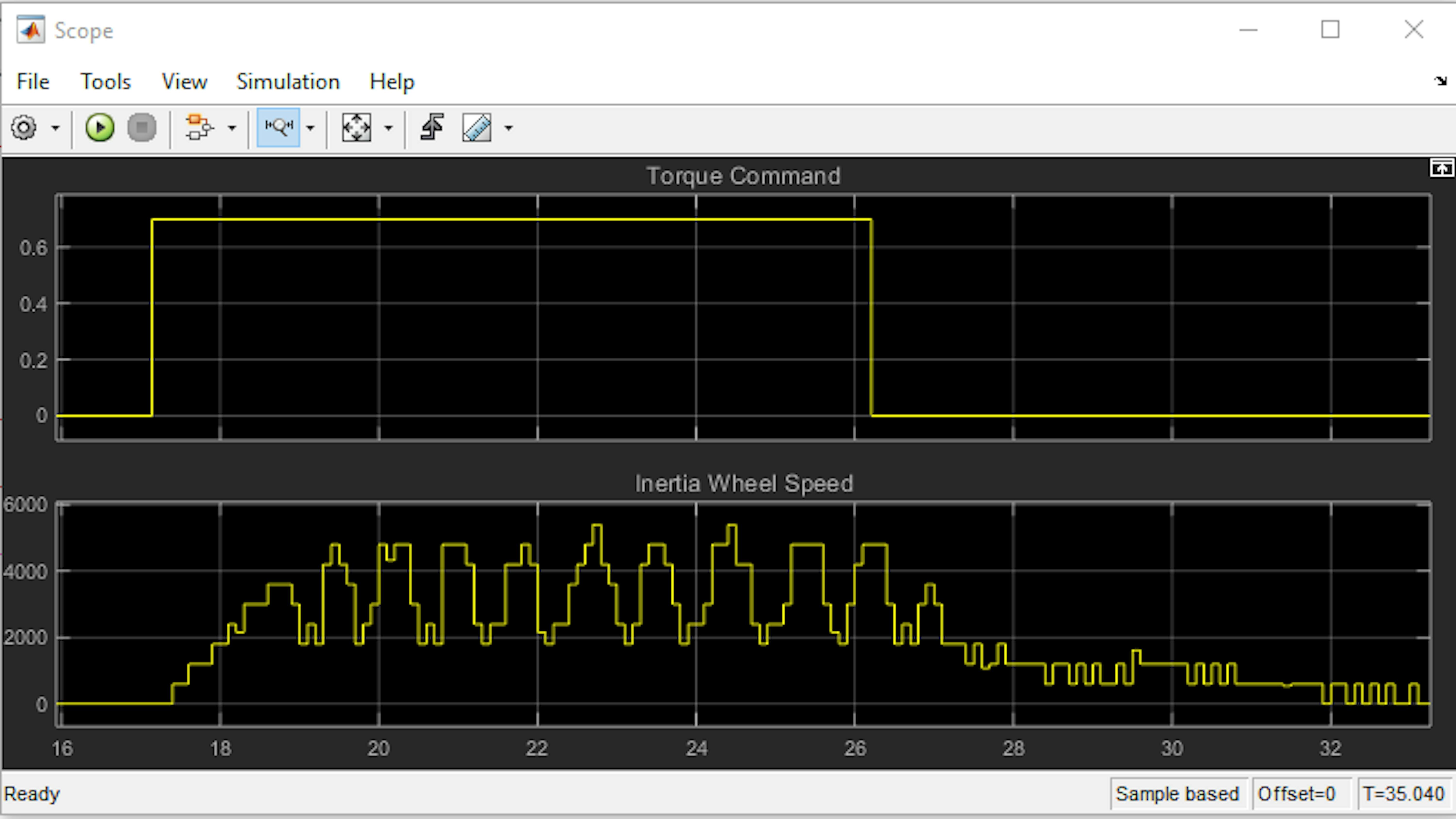
What happens to the motor when the speed threshold is exceeded? You will observe that the motor does not get switched off. Set the torque command to 0. In the figure above, you will see that instead of shutting off the motor permanently, it switches off each moment the inertia wheel speed exceeds the threshold and turns back on. By “permanently,” we mean until the application is restarted. This way you can give the DC motor and motor carrier some time to cool down before attempting to drive it again.
To do this, we will add a latch to the output signal from the Compare To Constant block. You want the Switch block’s control signal to be 1 if a high inertia wheel speed has never occurred and 0 if a high inertia wheel speed has occurred even once. To create the latch, add a Logical Operator block from Simulink → Logic and Bit Operations and a Unit Delay block from Simulink → Discrete. Set the logical operator to AND, set the initial condition of the unit delay to 1. Connect the blocks and label the output signal as shown:
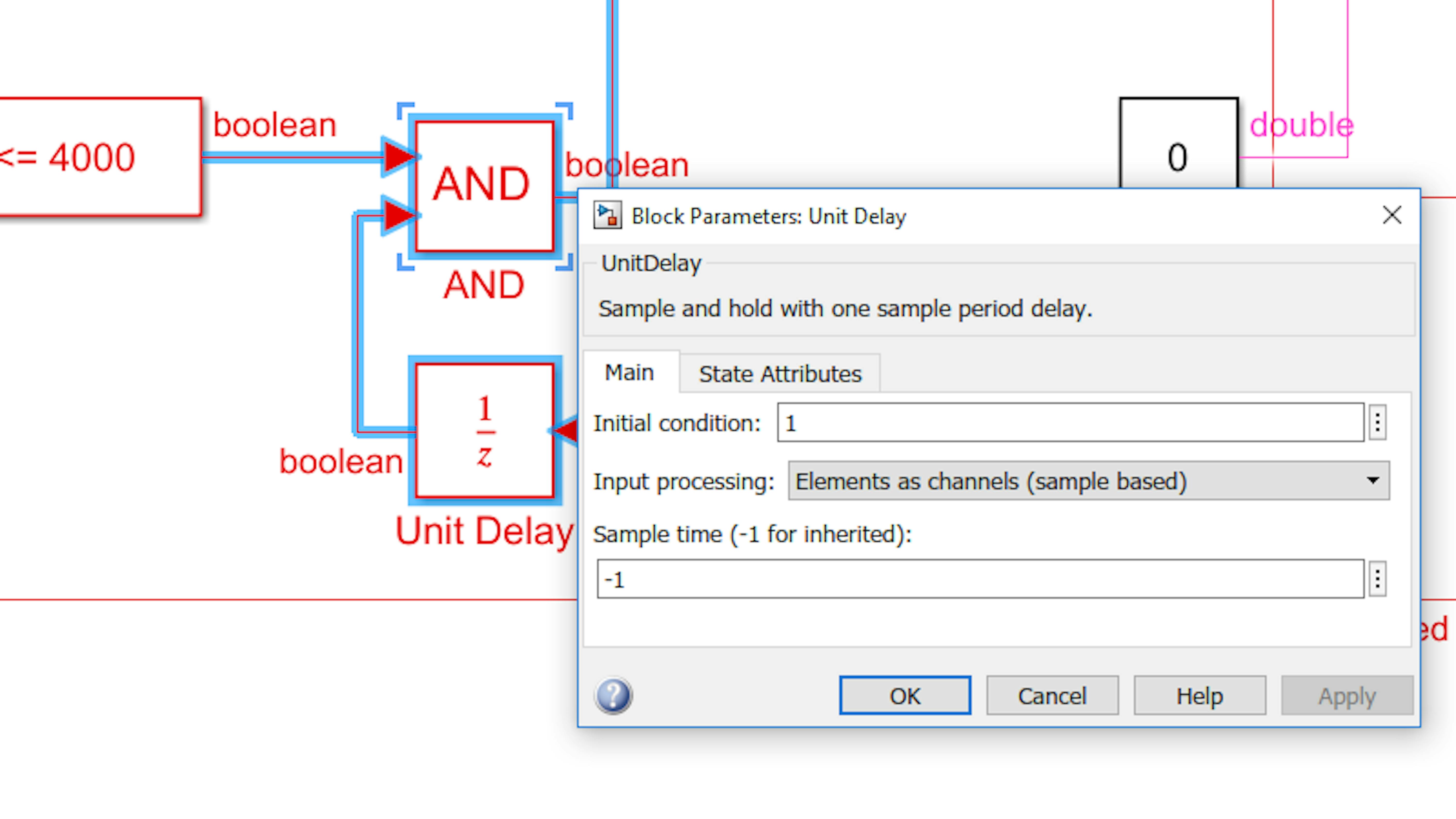
Note: The orientation of the Unit Delay block was reversed by clicking the block and pressing Ctrl + I.
Make sure you understand how this mechanism will permanently “latch” the Logical Operator block’s output to 0 the first time the speed threshold is exceeded.
Next, let’s create another subsystem to clean up the threshold and latch operations. Label the Inertia Wheel Speed signal as shown below. Select the Compare To Constant block, the relational Operator block, and the Unit Delay block; press the right-click button on any of the block and select Create Subsystem From Selection:
Label the subsystem as shown:
Now hold the motorcycle at the vertical position and run the model. Set the torque command to 0.7. Watch the Scope window and wait for the inertia wheel speed threshold to be exceeded. Does the safety mechanism work as intended now?
You might observe something similar on your scope.
Inertial Measurement Sensor - BNO055
To measure the lean angle θ and its time derivative θ˙, you will use an inertial measurement unit (IMU). On your motorcycle, you have a BNO055 9-axis absolute orientation sensor from Bosch. The BNO055 senses the gravitational vector and the magnetic field, and from those quantities it can determine rotational and translational motion. In this project, you will use the BNO055 to measure the orientation and angular velocity of the motorcycle about the wheel-ground axis.
See the full hardware specifications for the BNO055 IMU on its datasheet. It is important to get acquainted with datasheets as it is the way electronics are described. The blocks that we have prepared for you to use are constructed from these documents. Even if it is out of the scope of this course, you should keep in mind that it is possible to translate the information from a datasheet into a Simulink block to use it in your programs.
To test the BNO055 IMU, open the following model:
>> IMU0_start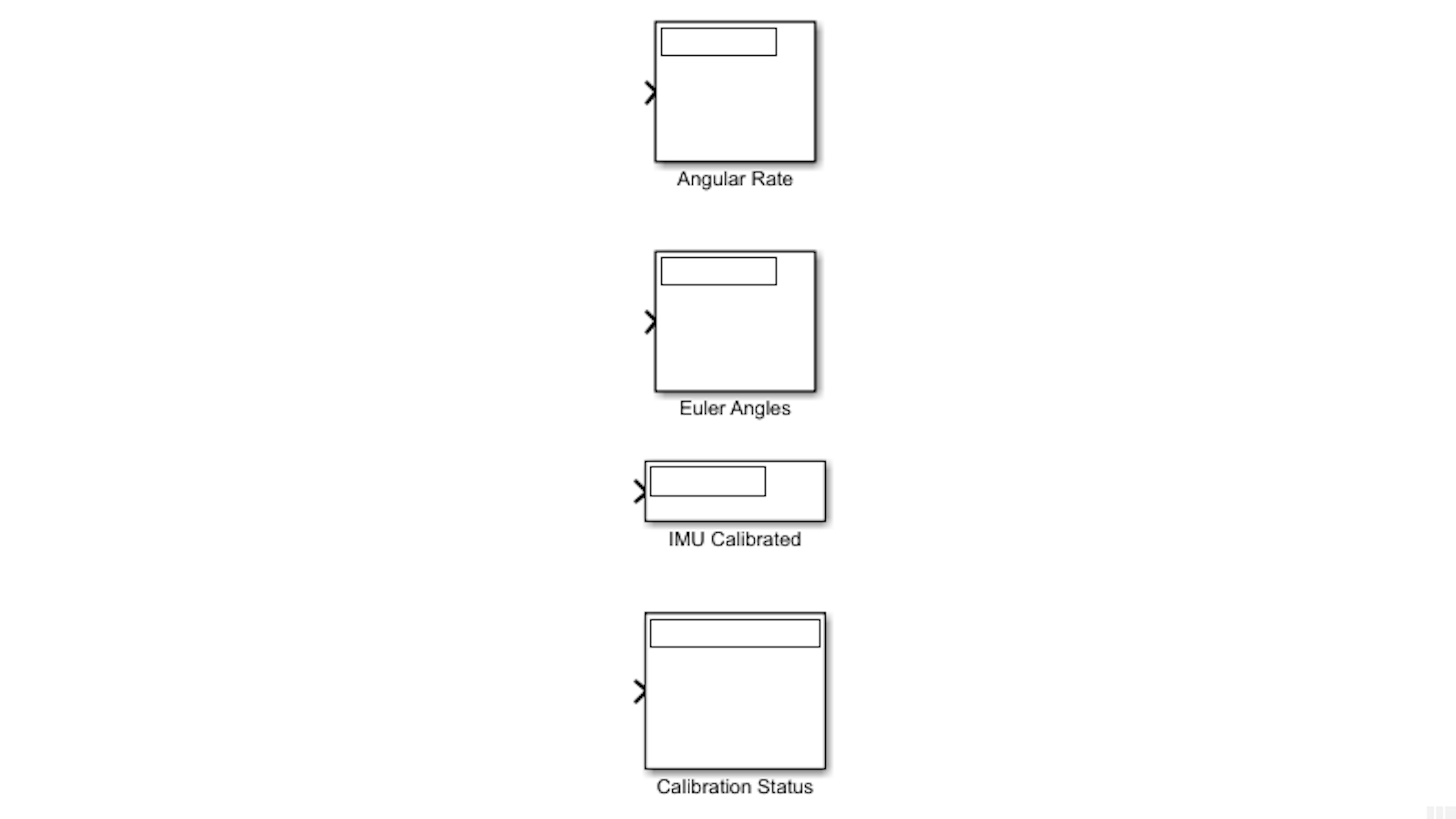
You will use this model to test the IMU, understand its outputs, and configure it for the motorcycle balancing controller.
Since you are going to be modifying the file, save the model as e.g. myIMU.slx.
In the Simulink Library Browser, locate the BNO055 IMU Sensor block in the Simulink Support for Arduino Sensors library and add the block to the model as shown in the next figure:
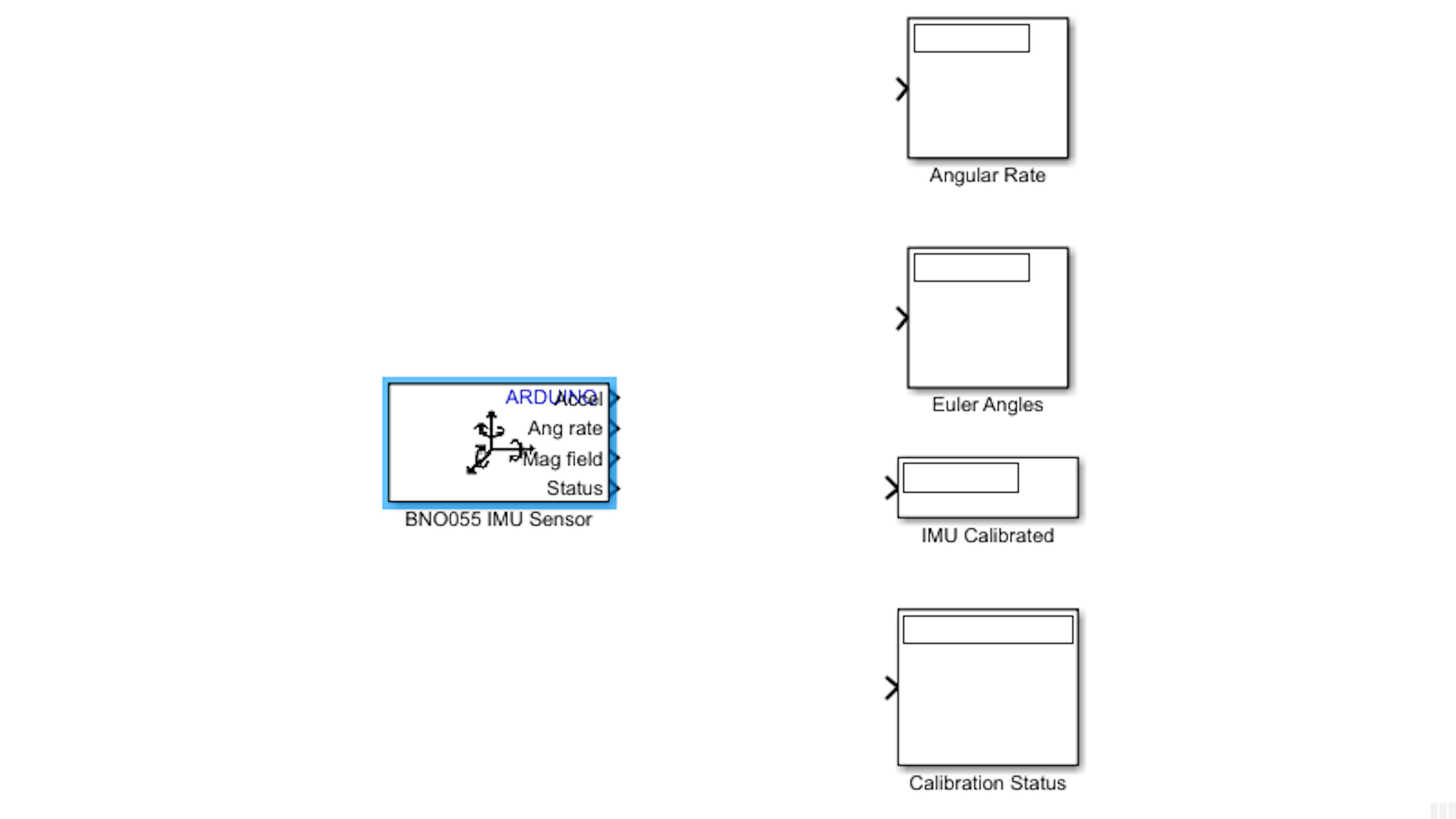
Open the block dialog window and examine the available options. Configure the block as shown:
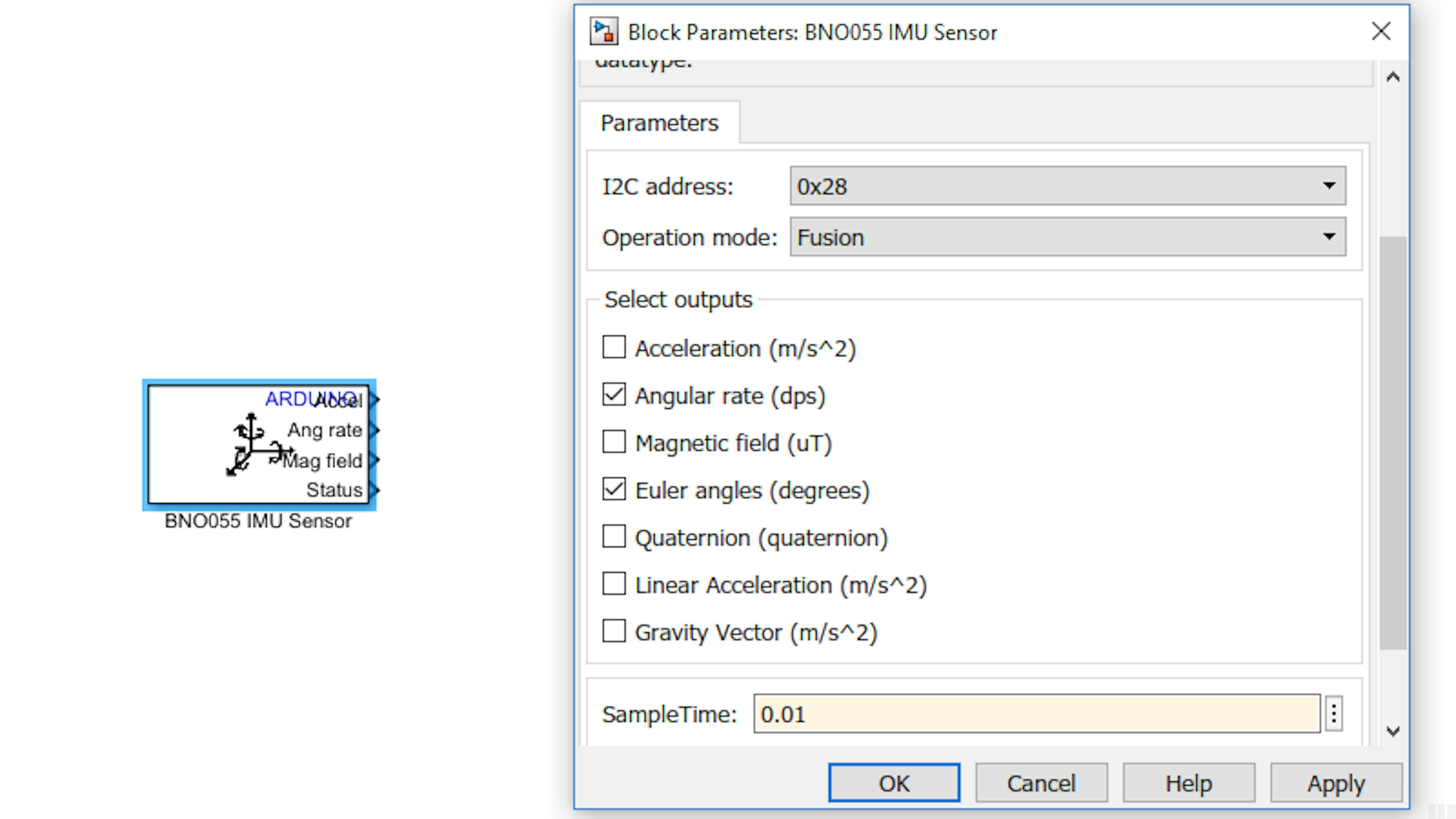
According to the chosen configuration, the block will output its absolute orientation relative to the magnetic field and gravitational vector as well as the angular rate along the local coordinates of the IMU sensor. The I2C address indicates which port the MKR1000 board will use to receive IMU data. I2C is a communication protocol that is implemented at the hardware level inside the Arduino controller. I2C is implemented in a bus format, which means that a series of devices can be connected on the same 2 pins from the microcontroller. The I2C standard allows up to 127 devices to be hanging from 2 wires and exchange data at relatively high speeds while keeping the wires between devices relatively short (in the range of centimeters). I2C devices, like the IMU used in this example, have specific addresses determined at the factory. When connected to the microcontroller, you will have to use the address to channel the data to and from that specific device. Addresses are expressed in hexadecimal format (0x28 in this case). Some devices allow changing the address, but some don’t. In our case, the IMU and part of the Motor Carrier are using I2C to communicate to the MKR1000.
Another option from the previous dialog window is the Sample time. In our case, the block needs to give measurements at 100 Hz (0.01 seconds) to react to the physical dynamics of the motorcycle with enough time for the motor to generate a corrective torque.
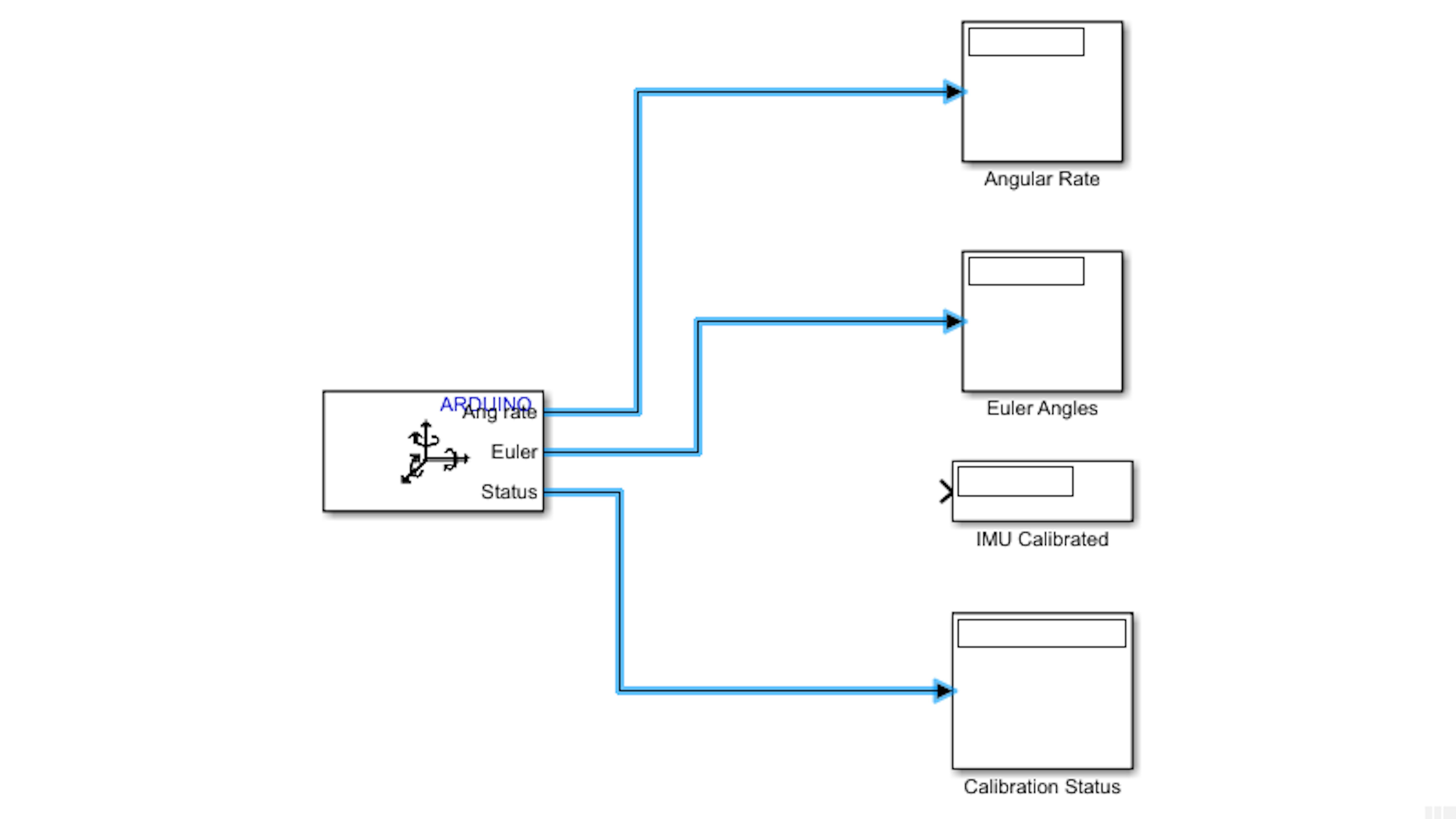
After configuring everything, click OK and return to the model window. Route the block outputs as shown:
Now, let’s try out the IMU! This model is configured to run in External mode, which means that it will be executed directly on your Arduino board, but it is meant to send information back to Simulink and display it on the screen. Click the Run button and watch the Display blocks.
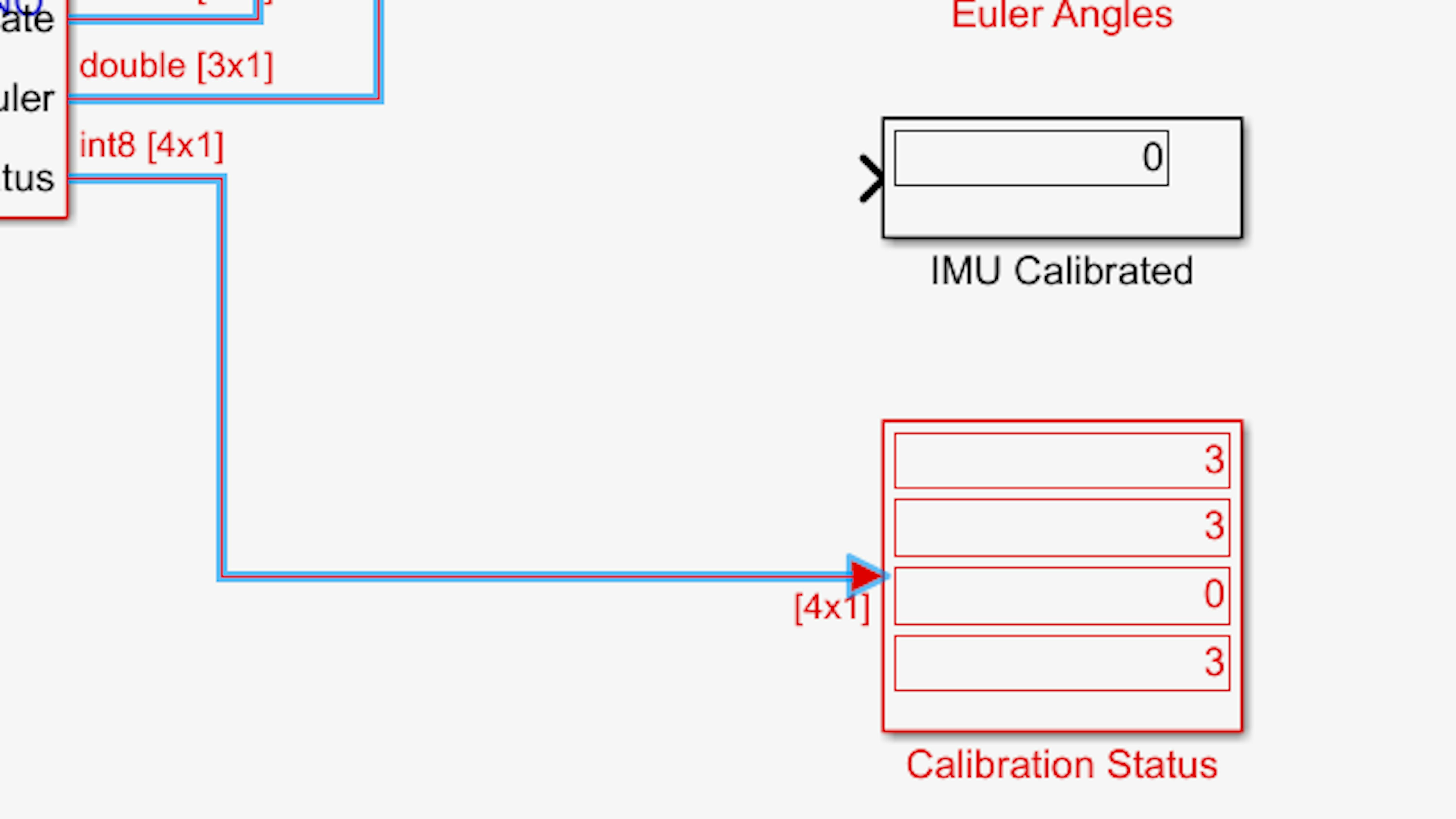
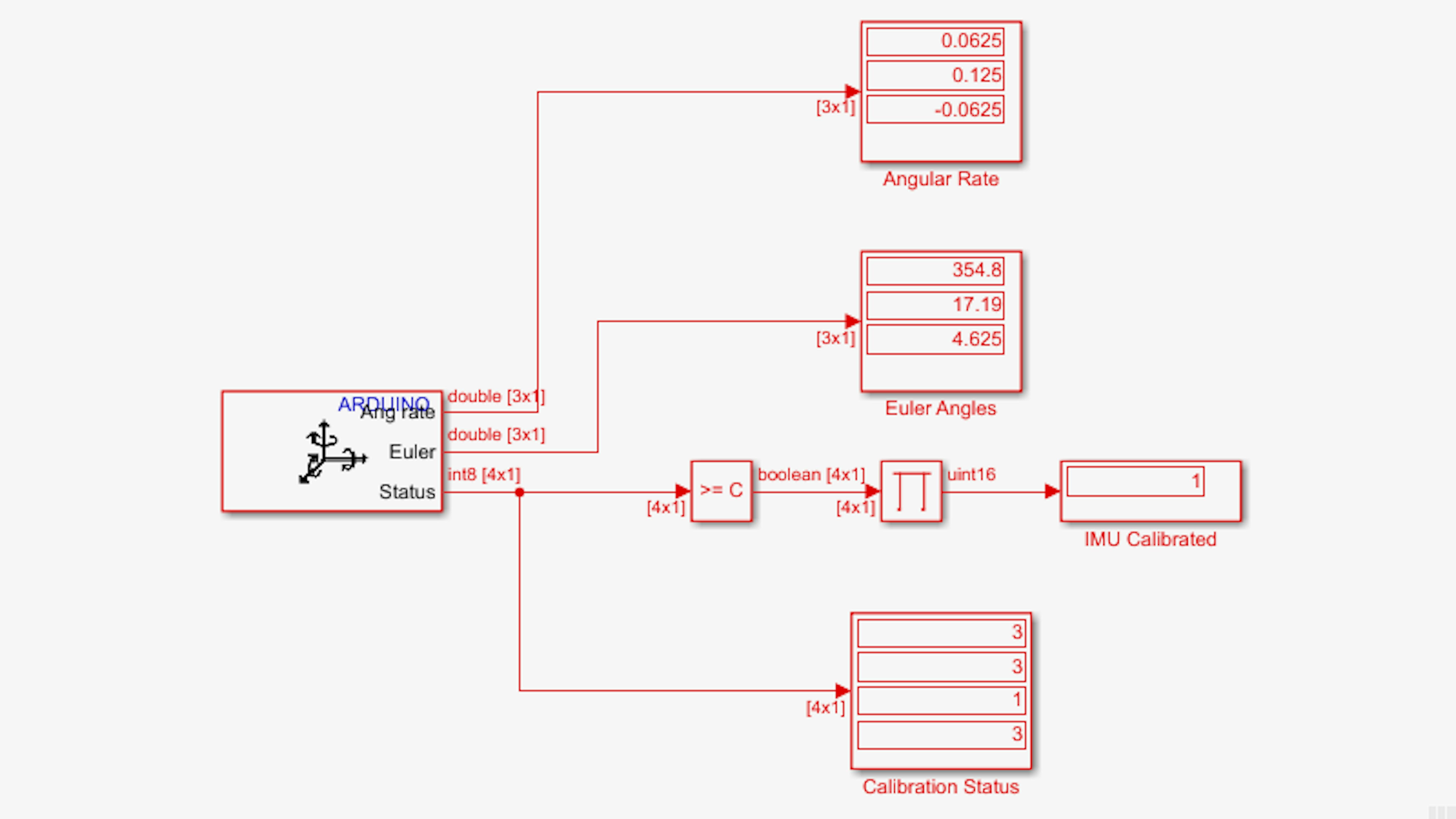
Examine the Calibration Vector display:
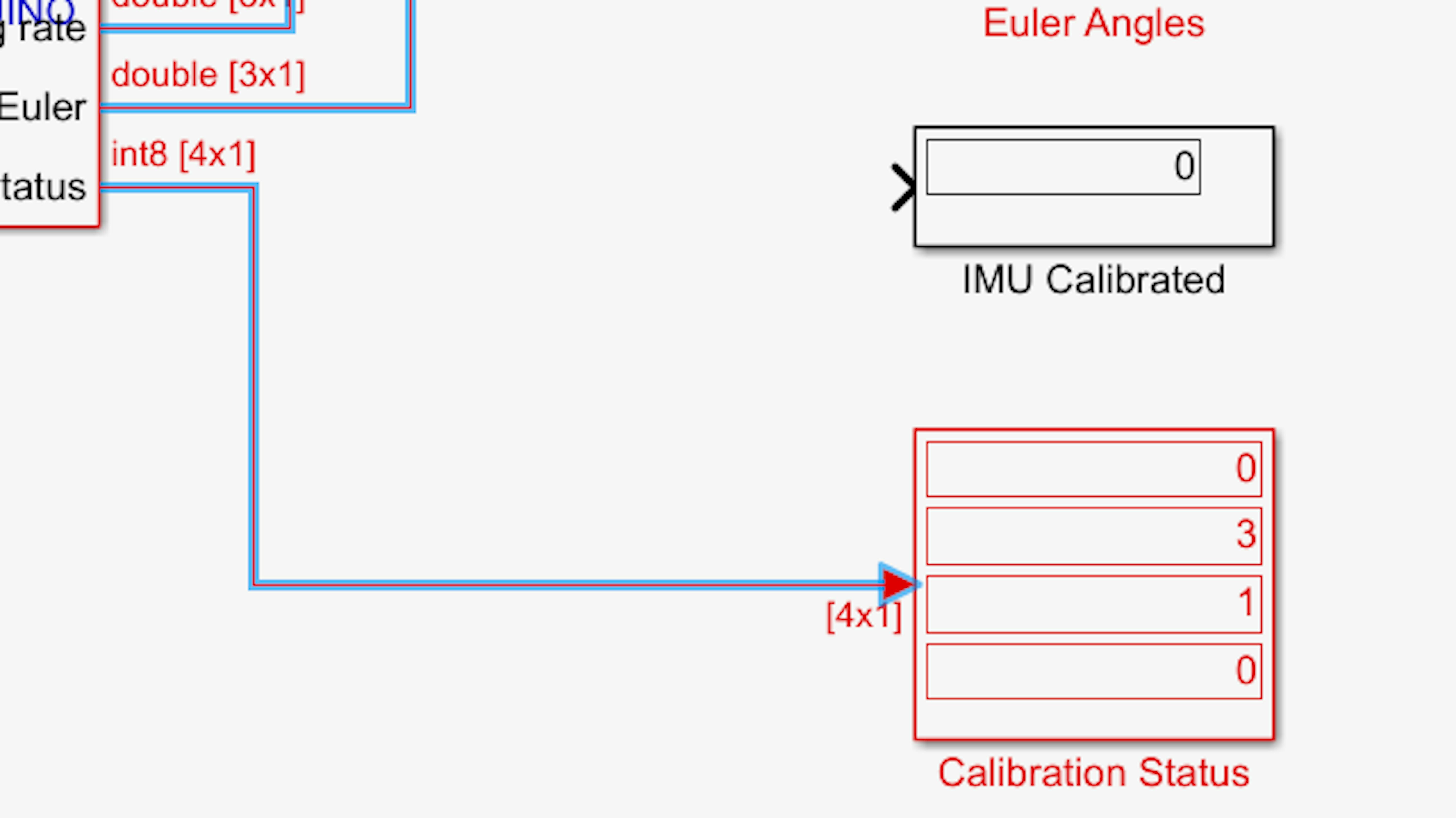
For the IMU to give accurate outputs, each sensor needs to be initialized to locate the gravity vector and magnetic field and offset the coordinates accordingly. The elements of the calibration status vector respectively represent:
- IMU system
- Gyroscope
- Accelerometer
- Magnetometer
Each calibration status vector element has a value of 0 to 3, indicating the degree to which the sensor is calibrated. For the motorcycle, you need the gyroscope and the magnetometer to be fully calibrated (3). Calibrating the IMU takes some practice. To start, leave the motorcycle completely at rest while the model runs in External mode. This should calibrate the gyroscope. Next, pick up the motorcycle and rotate it at least 90 degrees along each of the 3 spatial axes.
The previous operation should calibrate the magnetometer.
This calibration process must be done every time the BNO055 IMU is powered on, which means that you will have to figure out strategies in your model that will include calibration for those times when you power up your motorcycle. Now, let’s look at the rotational measurements. Examine the Euler Angles display:
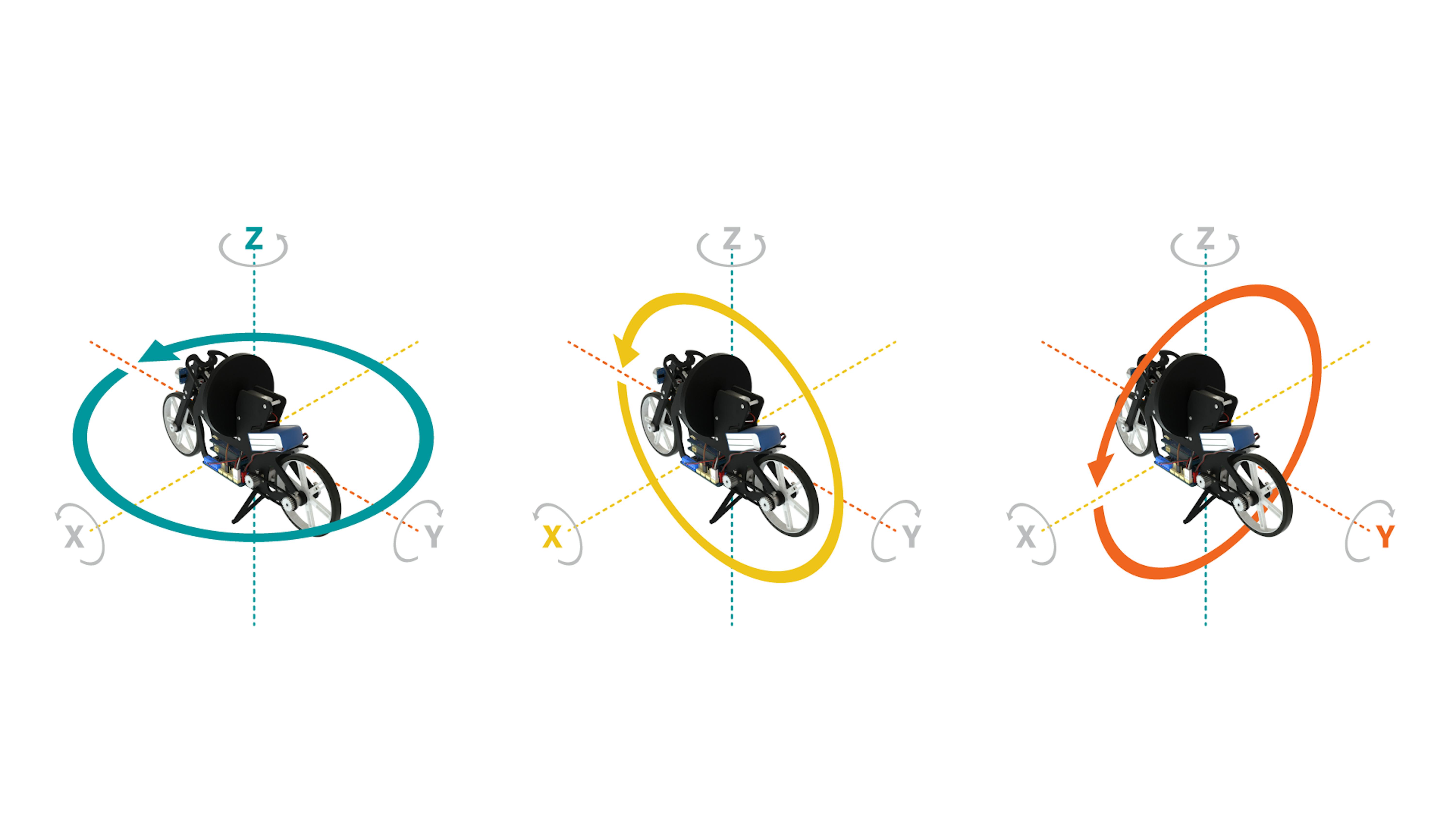
Try rotating the motorcycle along each axis, and identify which angle corresponds to each motorcycle axis. Which element of the Euler angle vector represents the lean angle θ? You should observe that the second Euler angle responds most noticeably to changes in the lean angle.
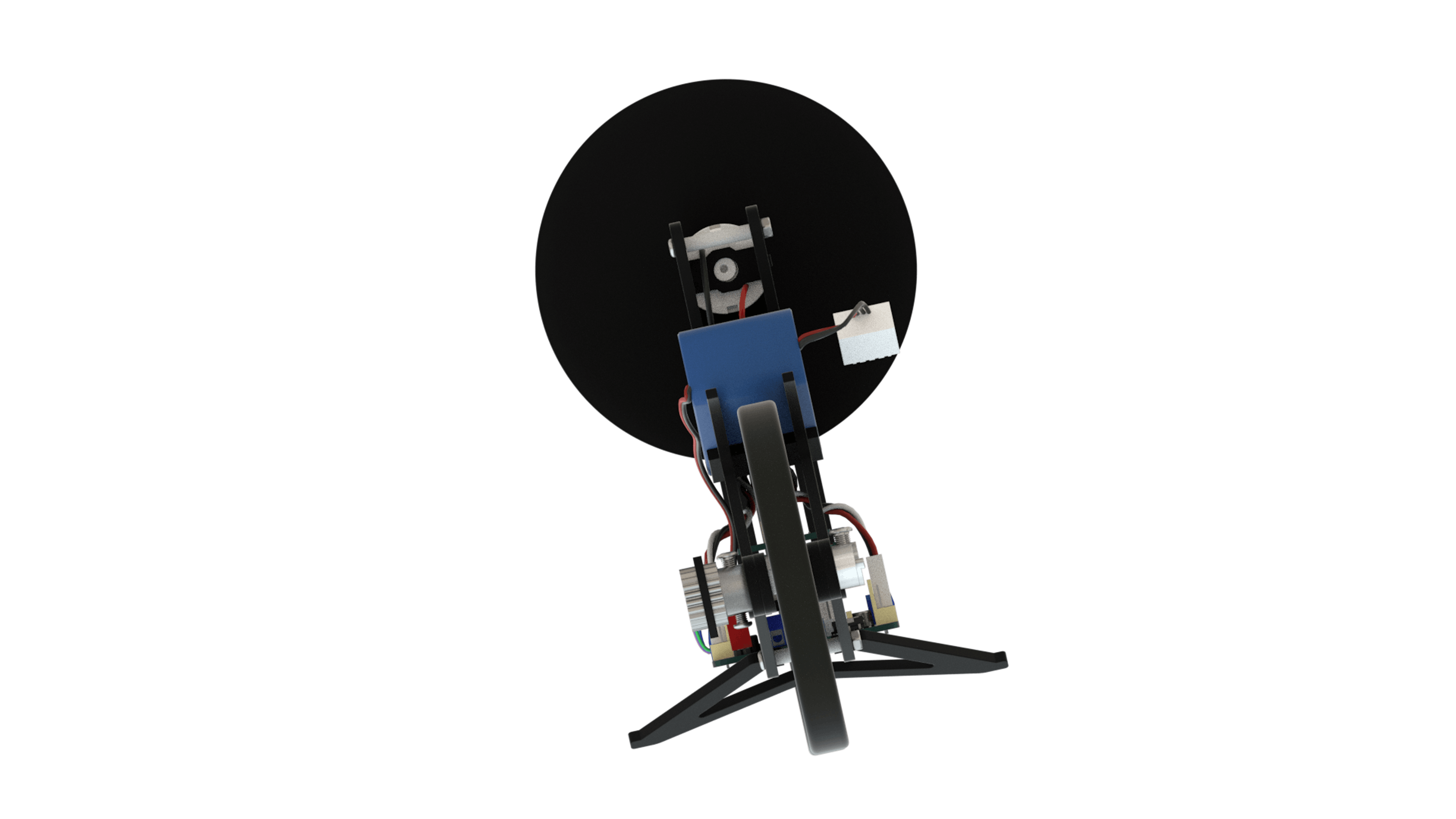
Orient the motorcycle so that you are looking at the back of the inertia wheel.
Roll the motorcycle about the wheel-ground axis. In which direction does θ increase (clockwise or counterclockwise)? You should see that θ increases as you lean the motorcycle counterclockwise.
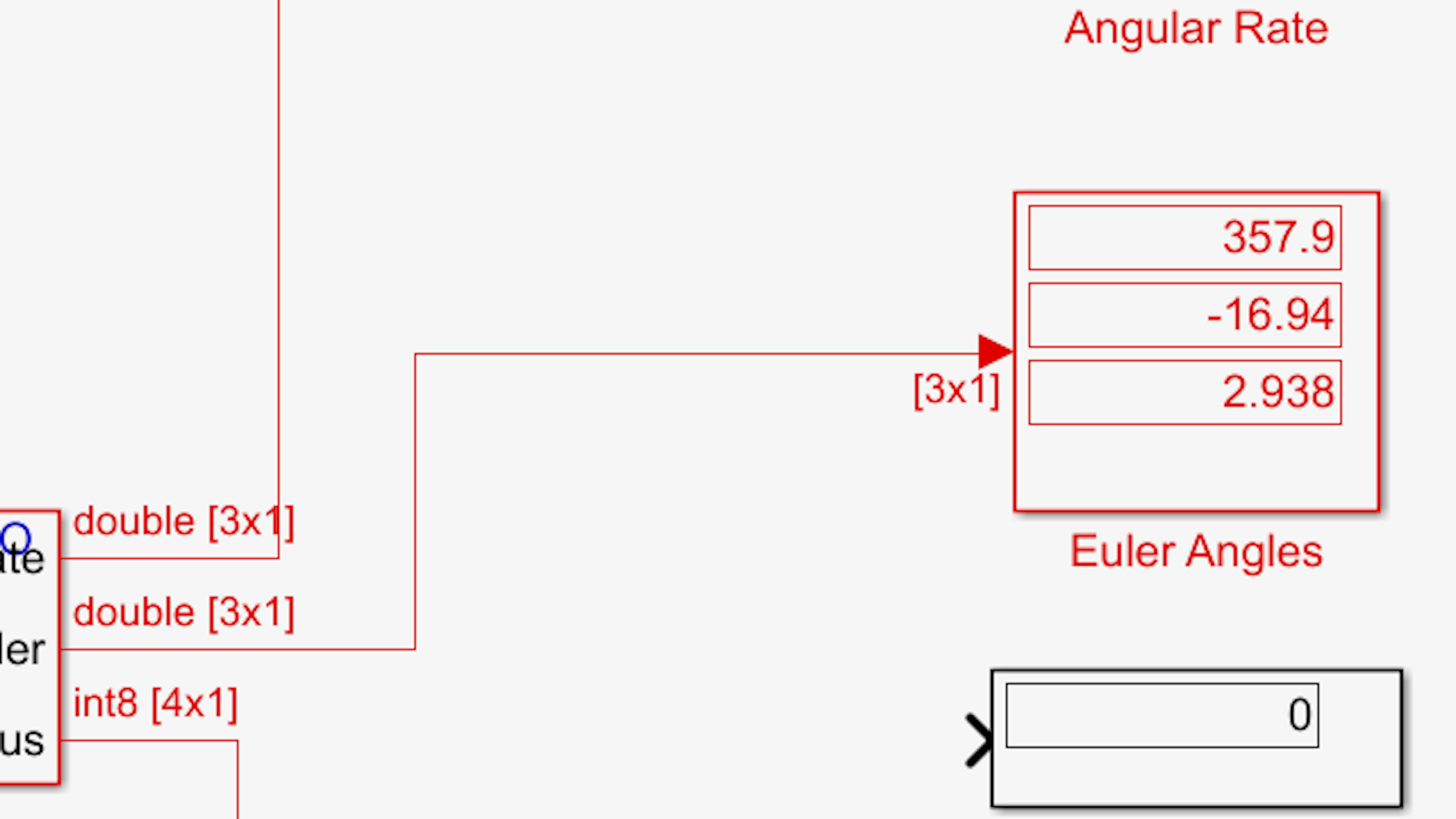
Now observe the Angular Rate display:
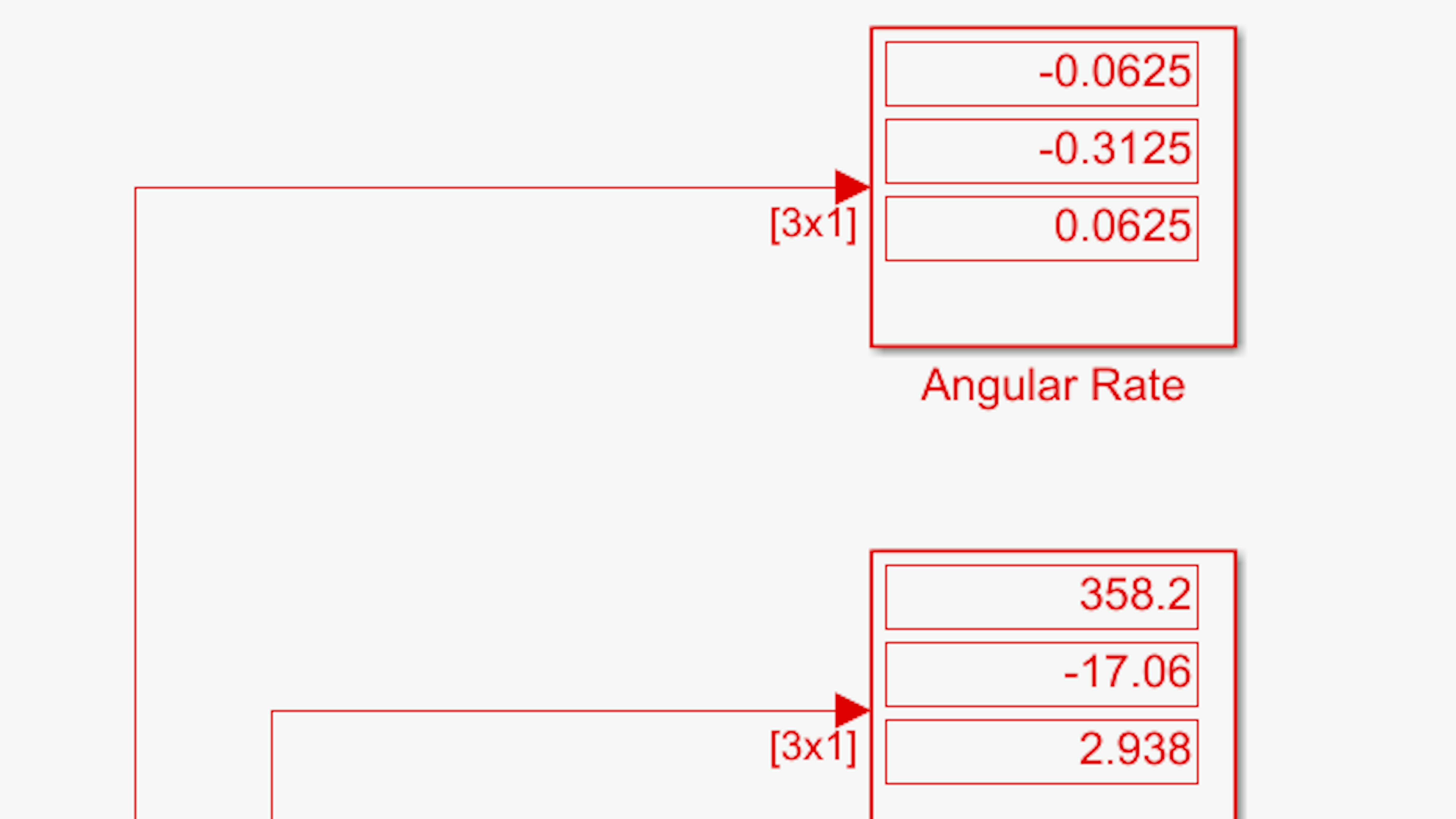
Using a steady motion, rotate the motorcycle along the wheel-ground axis. Which element of the angular rate vector represents θ˙? In which direction is the angular rate of that vector element positive (clockwise or counterclockwise)? You should observe that the second angular rate vector element represents the lean angle rate and that it shows a positive value for clockwise rotation about the wheel-ground axis.
It may seem mysterious that as θ increases, θ˙ appears to be negative. It is because the Euler angles show absolute orientation with respect to the fixed inertial frame (defined by the gravitational vector and magnetic field), while the gyroscope measures rotational velocity in the IMU’s reference frame. Thus, from the IMU’s perspective, the rotation measurement is the opposite of how you view it from the fixed inertial frame.
Once you have become familiar with the different angular measurements, stop the model and let’s look at how to tweak the model to extract the information in the format we need it for our controller.
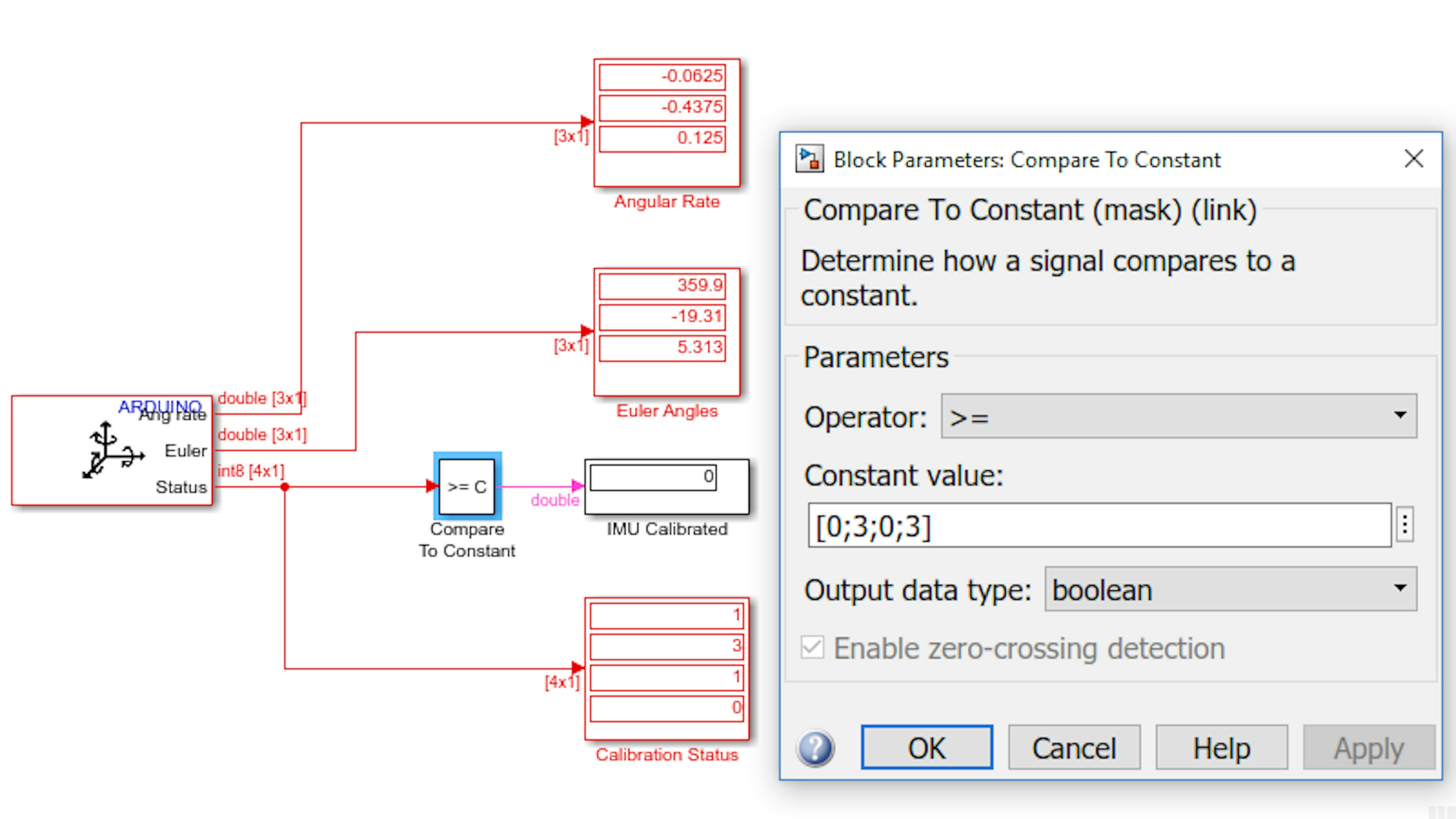
Given the outputs of the BNO055 block, let’s manipulate them to get the information you need for balance control. First, let’s simplify the process of checking the calibration status. You can define the minimum calibration status as a 4x1 vector: [0;3;0;3], which, compared to the vector signal coming out from the sensor, would give a much simpler answer to the question “is the sensor calibrated?” Add a Compare to Constant block from the Simulink → Logic and Bit Operations library to the signal giving the calibration information. Connect and configure the block as shown:
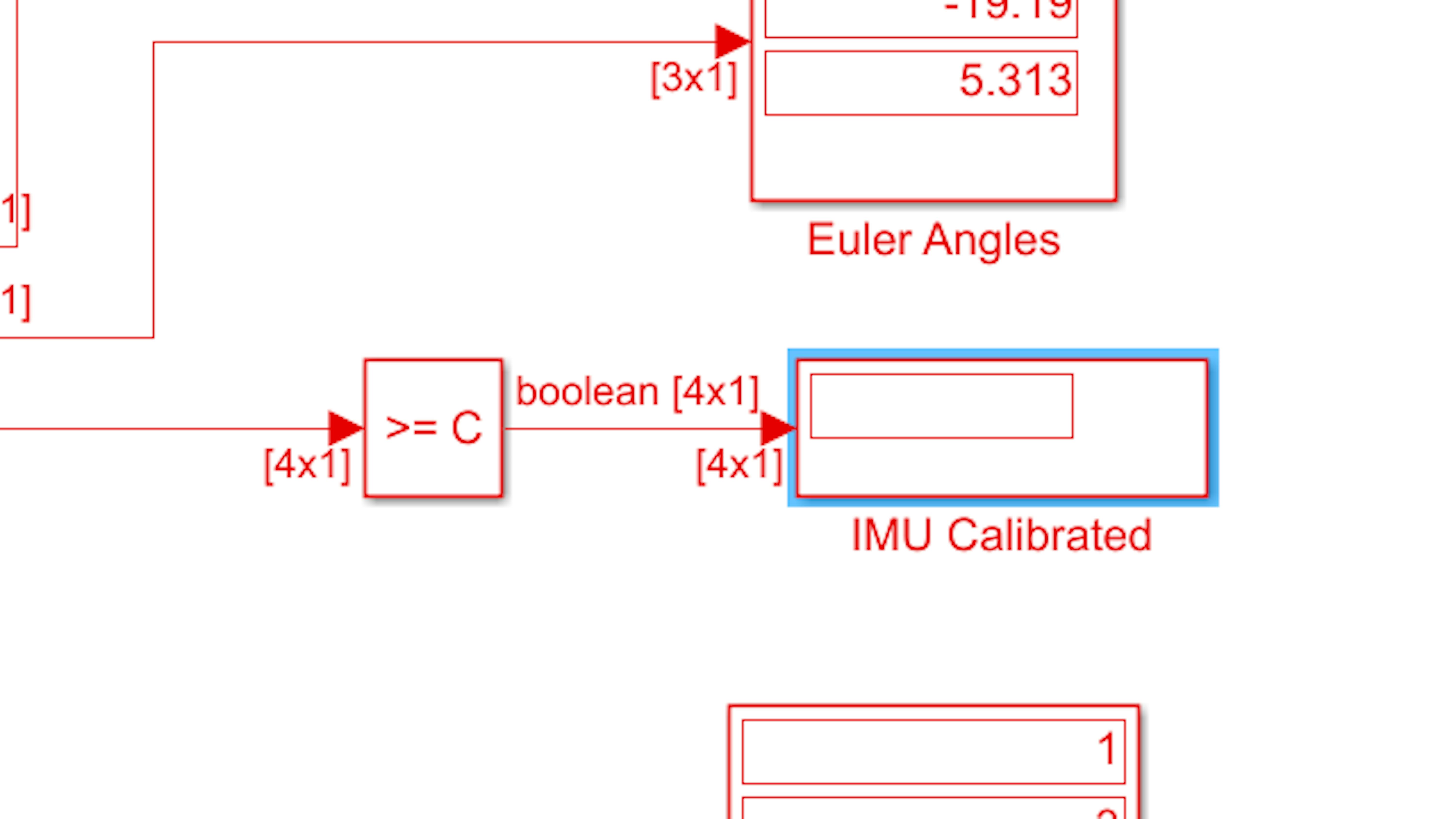
Update the model diagram by pressing Ctrl+D. Examine the dimensions of the Compare to Constant block output. Is this what you want?
Rather than seeing whether each of the sensor components are sufficiently calibrated, you want to know whether all the sensor components are sufficiently calibrated. Add a Product of Elements block from Simulink → Math Operations and insert it between the Compare to Constant block and the Display block:
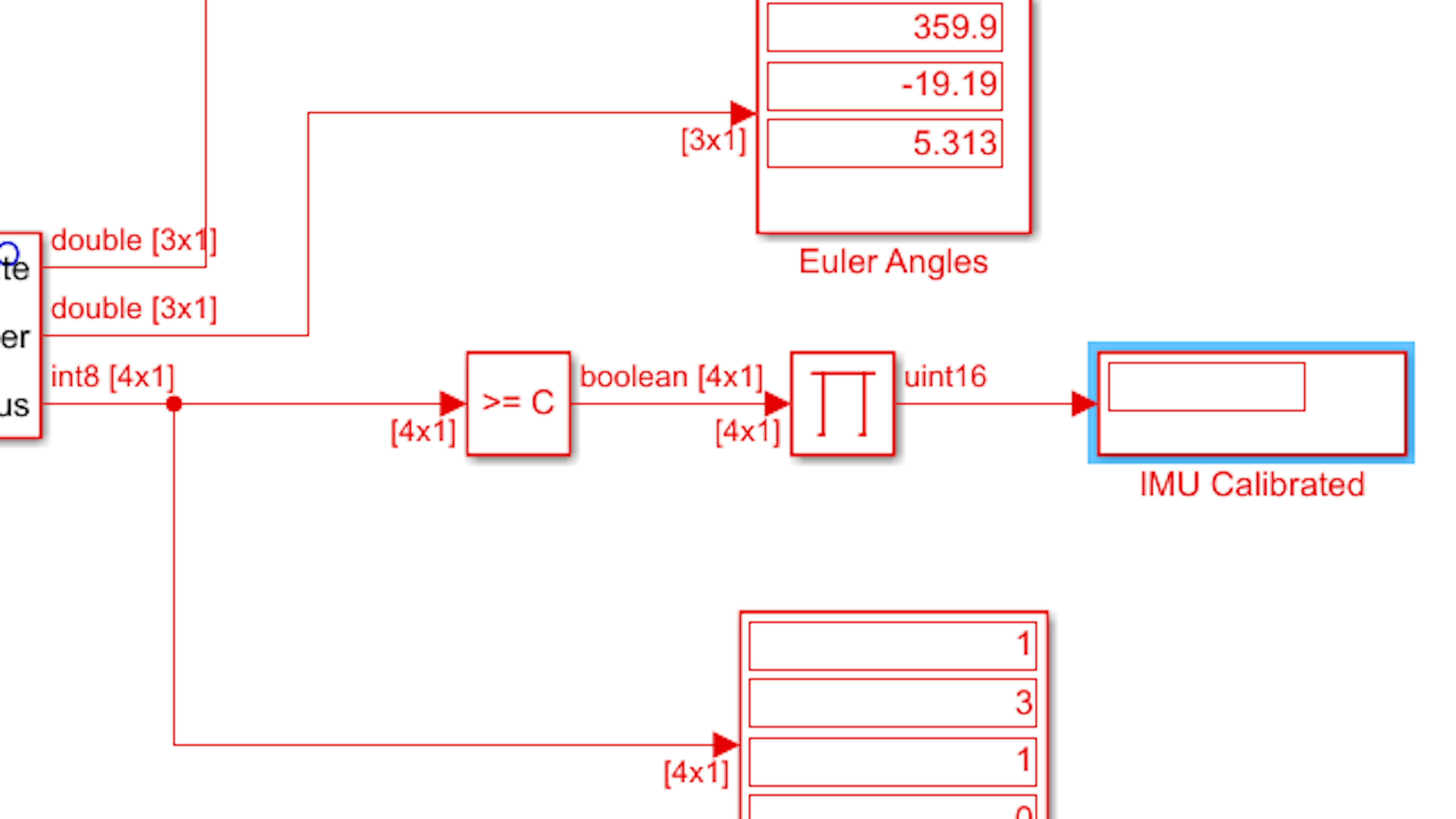
Run the model and confirm that you get a single true or false value to indicate the calibration status of the IMU:
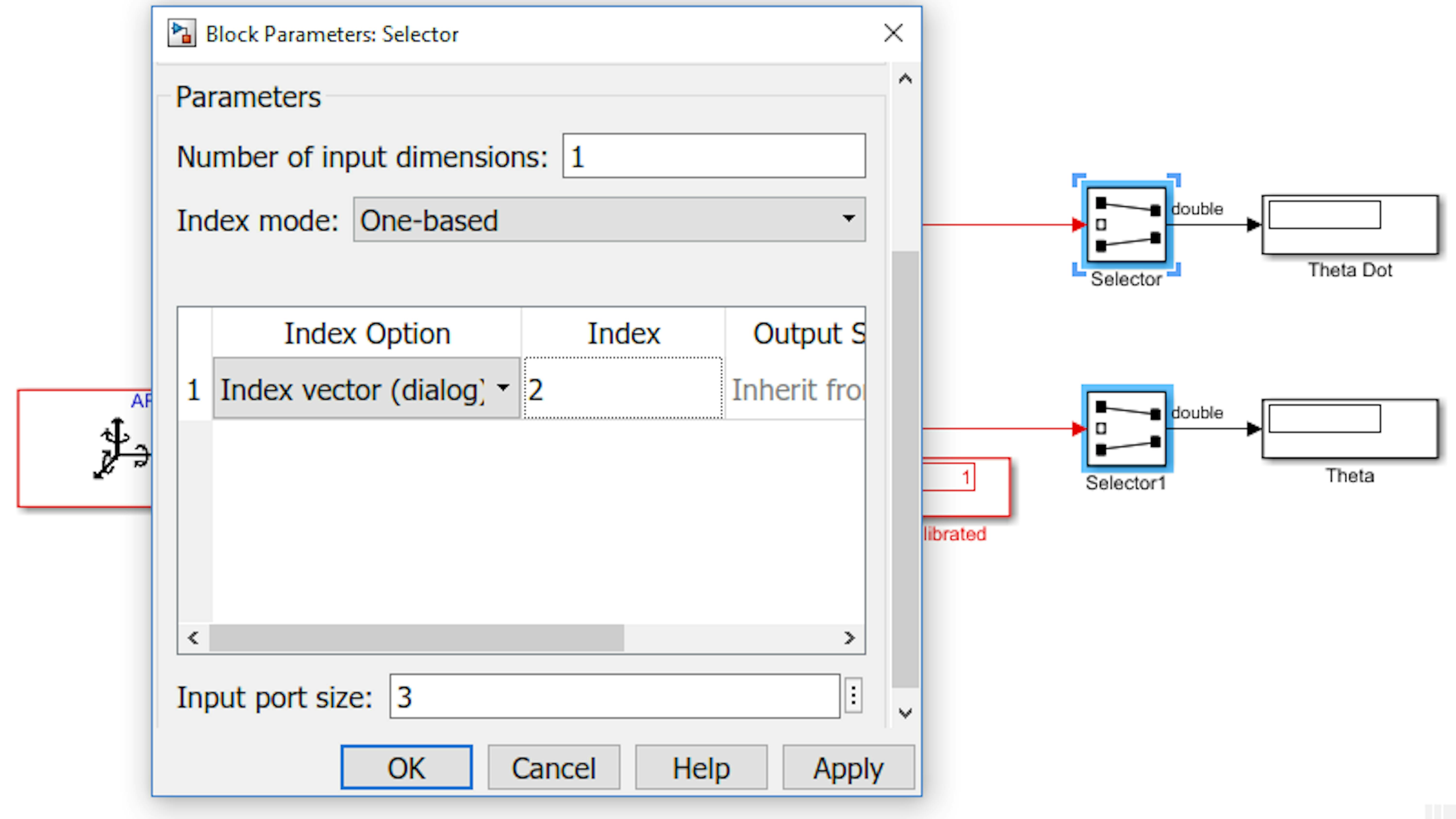
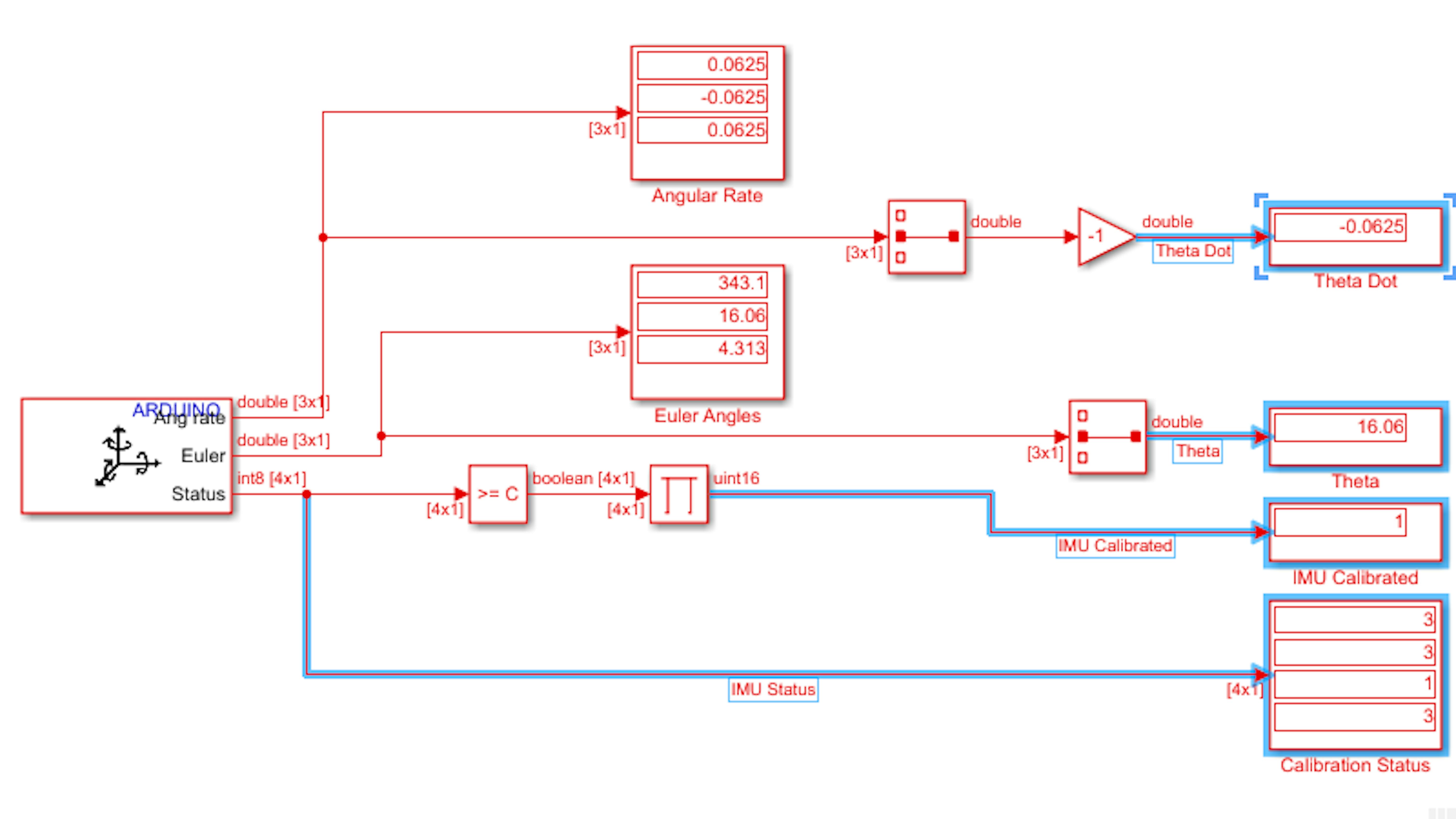
Next, let’s isolate the rotational measurements you want for the motorcycle. To index into a vector signal in Simulink, you can use the Selector block. Locate the Selector block at Simulink → Signal Routing and add two of them to the model. Then, find the Display block in Simulink → Sinks and add two of them to the model. Route the signals as shown:
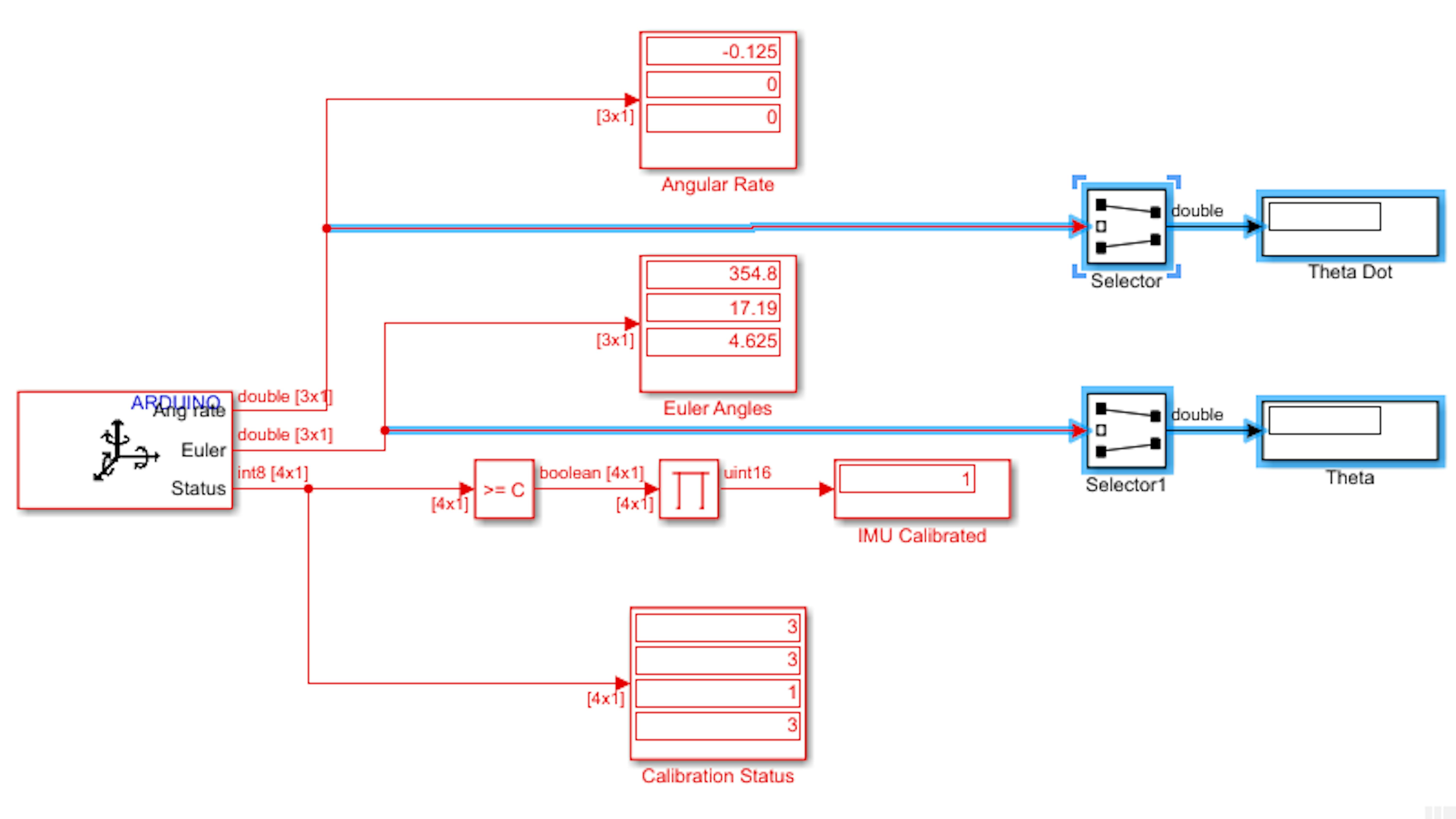
Configure both the “Theta Dot” and “Theta” Selector blocks with an index of 2 as shown in the following screenshot:
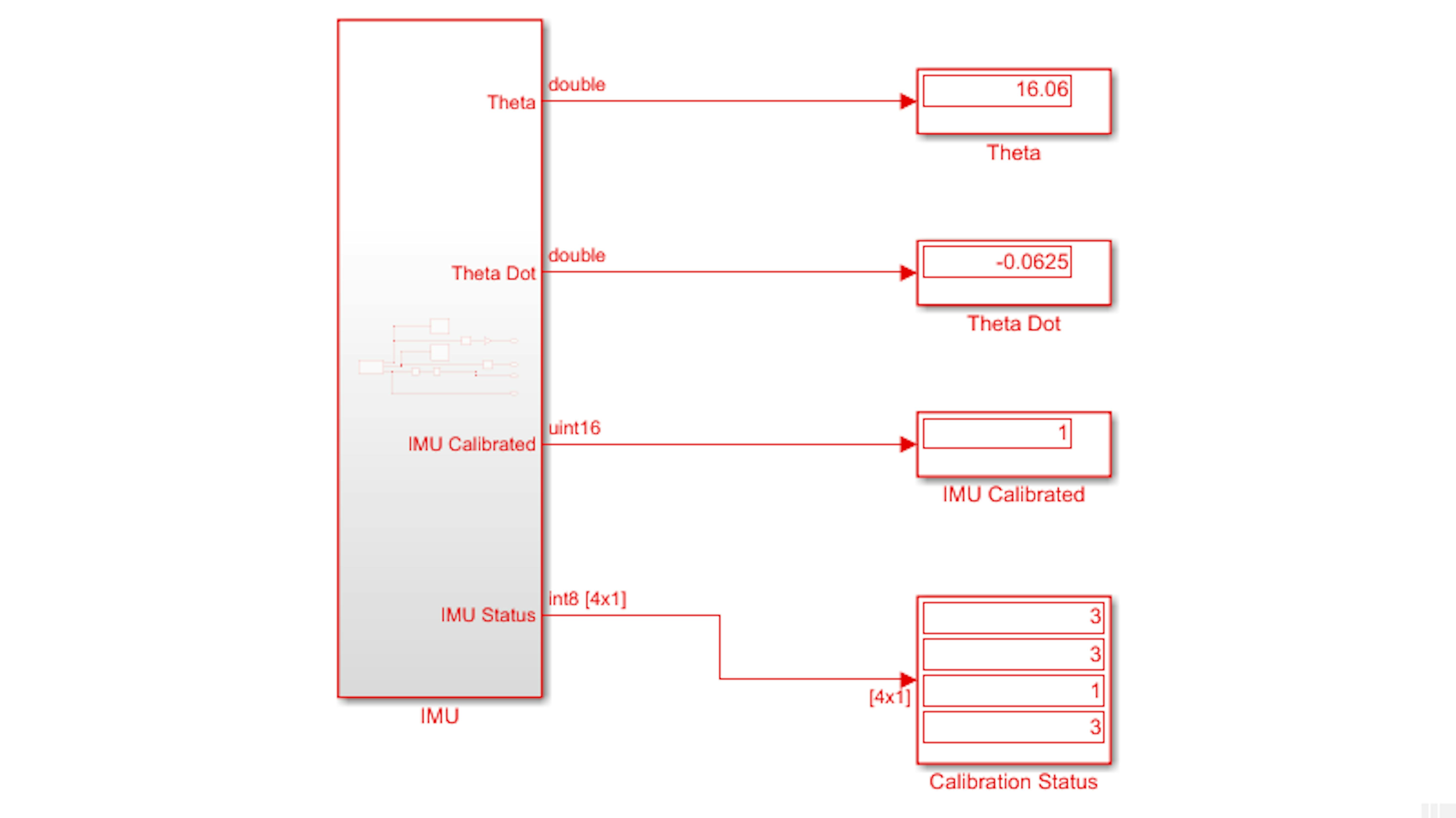
Run the model and confirm that the Display blocks show θ and θ˙, as you defined them:
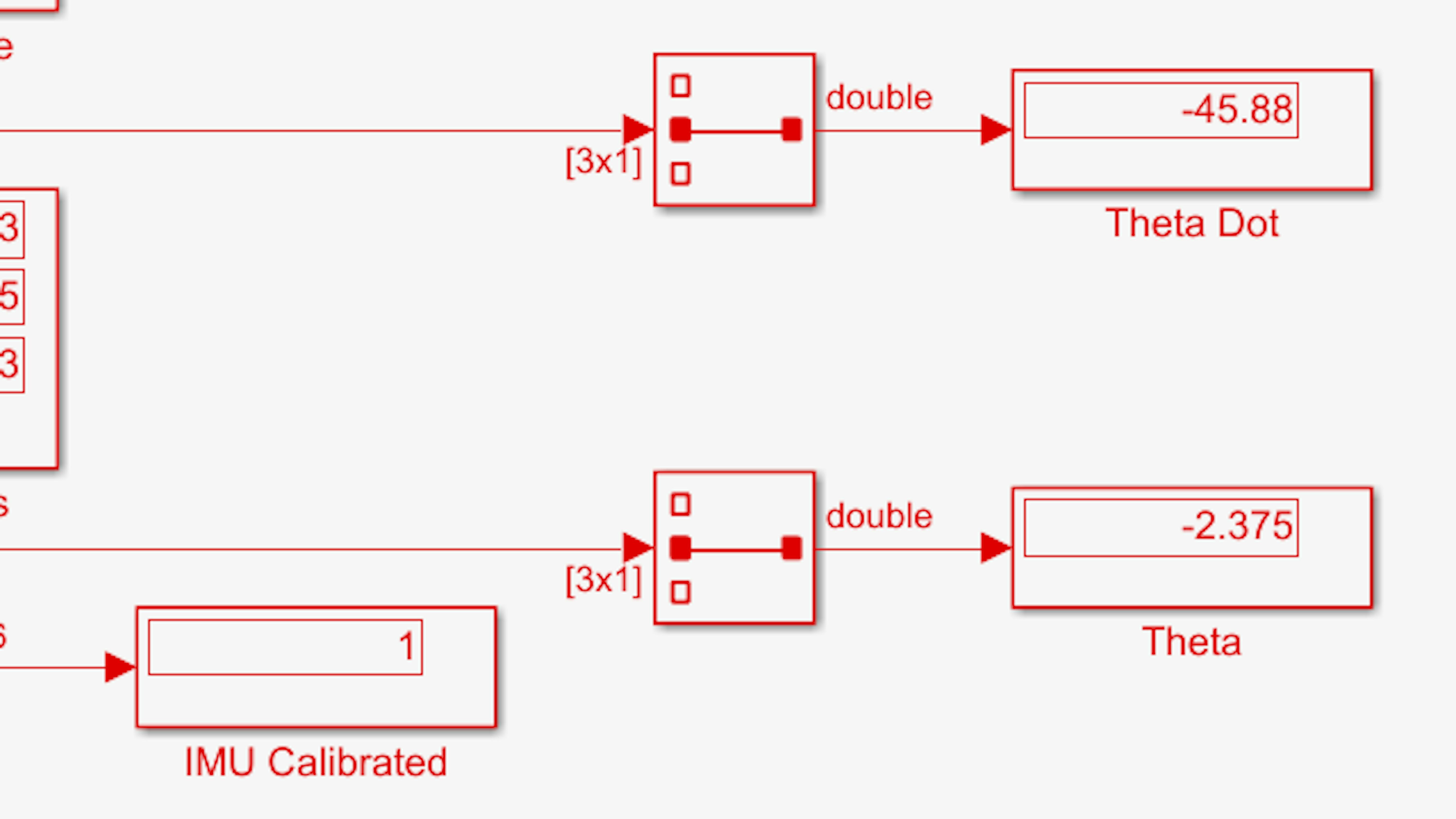
Let’s just take care of one more detail. For the purposes of this project, you want θ and θ˙ to be defined with the same polarity, but the BNO055 IMU defines them with opposite polarity. Add a Gain block along the “Theta Dot” signal path, and set the gain value to -1:
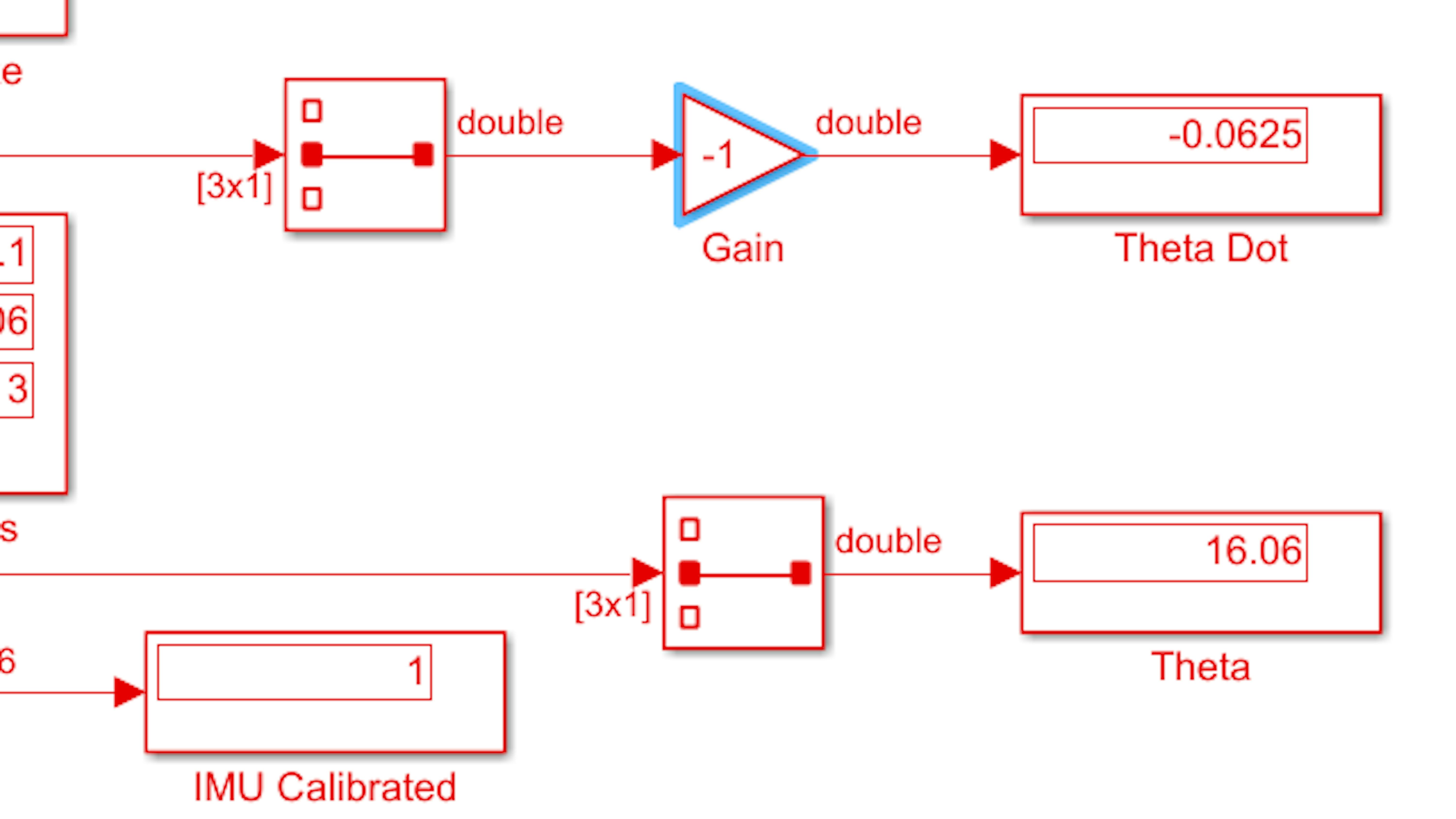
Run the model once more to confirm the correct behavior of the signal conditioning for θ and θ˙.
Stop the model when you are finished, and let’s do some rearranging of the model so that it will be easier for you to incorporate this work in later designs.
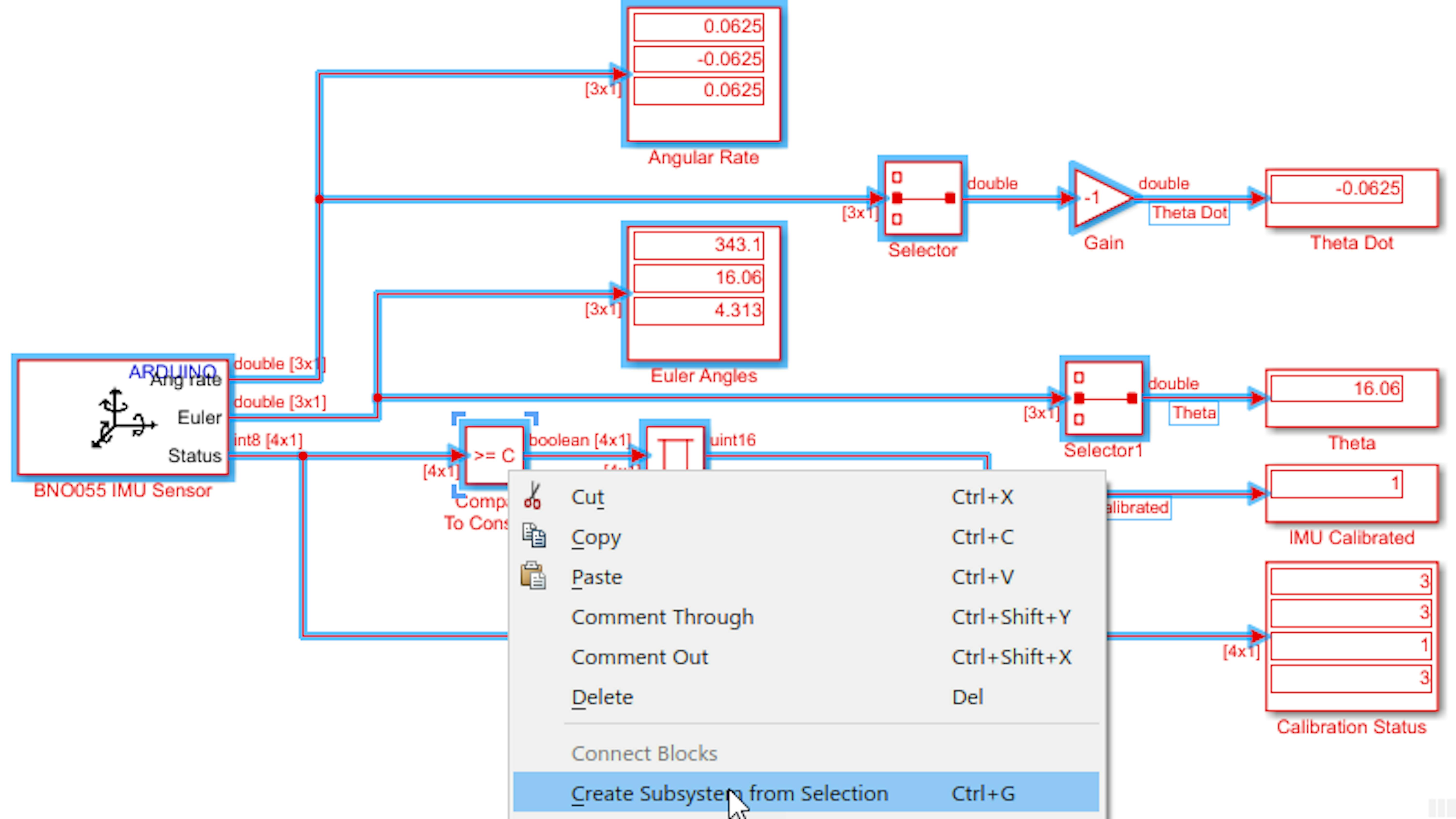
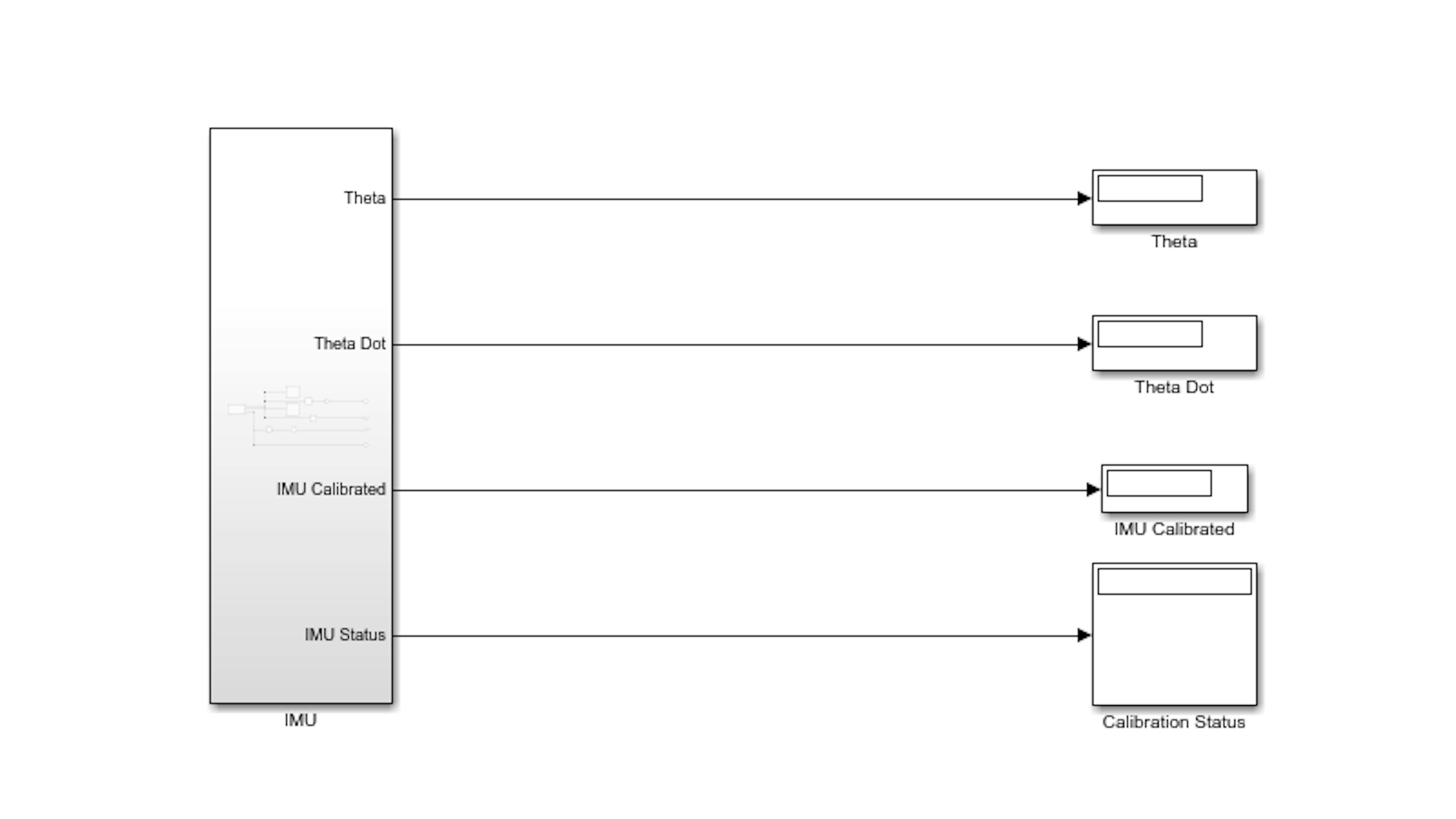
Make an IMU subsystem to use in the motorcycle model later. Move the Theta Dot, Theta, IMU Calibrated and Calibration Status display blocks so that they are vertically aligned on the far right of the block diagram. Then, label the 4 output signals as shown in the image: Theta Dot, Theta, IMU Calibrated, and IMU Status.
Highlight everything in the model except the 4 right-most Display blocks (the ones you just aligned to the right), right-click on a selected block, and select Create Subsystem from Selection:
For modeling convenience later, the subsystem’s first output should be Theta and the second output should be Theta Dot. You can change the port order by adjusting the Port number property in the subsystem’s outport blocks. Go inside the new subsystem and double-click the Theta Dot outport block. Set the port number to 2. The following image highlights the second part of the process:
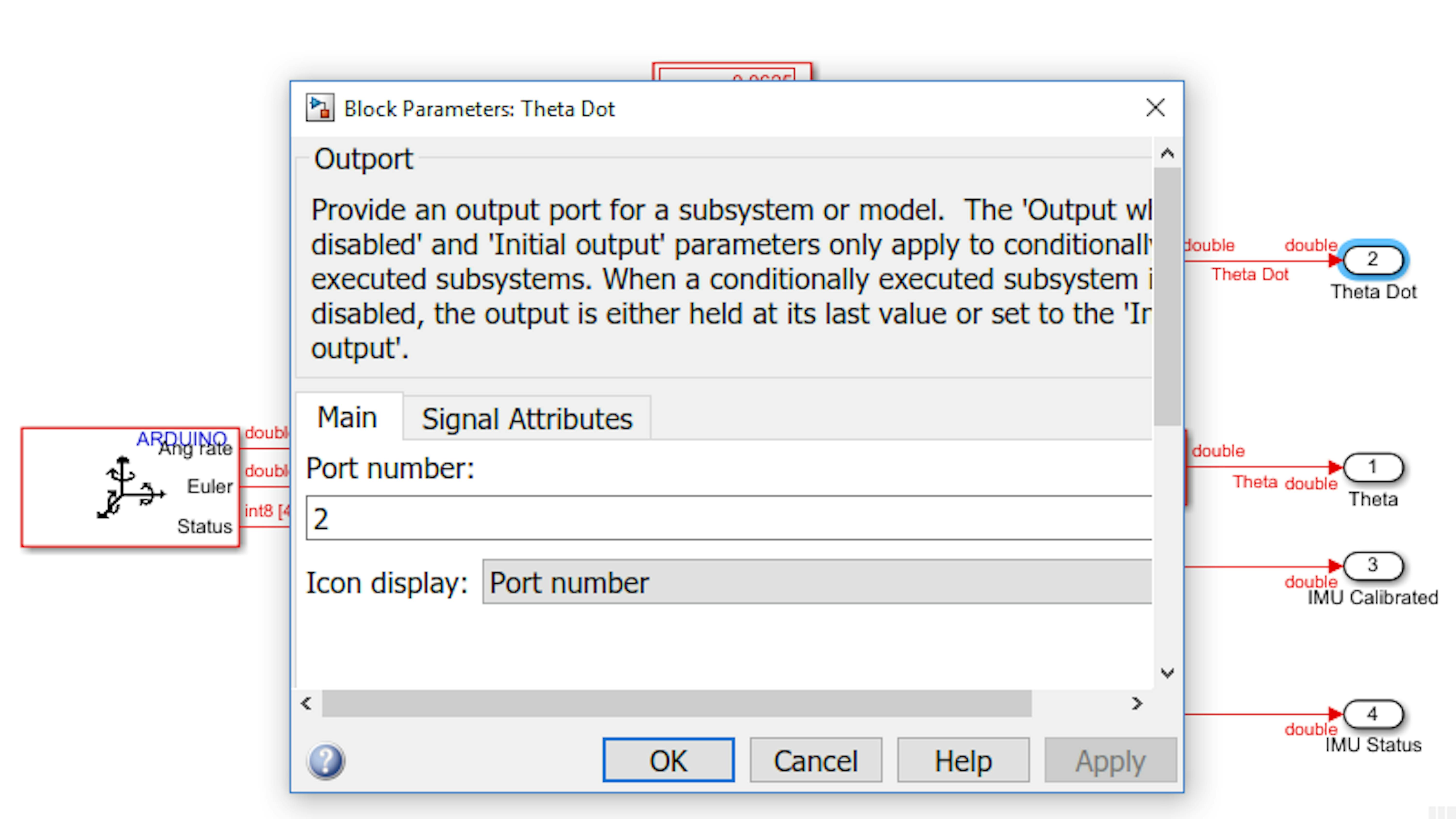
Next, clean up the model’s layout and label the new subsystem block IMU:
When running a model in External mode, you must be careful to manage how much signal data you observe using Scopes, Displays, or any other simulation-time signal monitoring features. In External mode, all “observed” signals transmit serially from the external hardware through the USB cable to your computer in real-time. There is an inherent limit to the number of bits per second that can be transferred in this manner and exceeding this limit will slow down the simulation. Therefore, you should only activate Displays and Scopes on the signals that you need to observe for a given purpose. For the current model, you will not hit this limit, but you should keep this potential issue in mind for other experiments you might be conducting. You can also bring signals of interest to a slower sample rate to meet serial communication limitations or transmit signals over an alternative communications channel such as Wi-Fi.
Finish the experiment by saving your model. It is now ready to be used within the project.
LEARN BY DOING
In this section, you learned about the tachometer and how it can be used to limit the rotation speed of the inertia wheel as well as the inertia wheel motor itself. Furthermore, you got to know more about the IMU sensor included in the kit and how it relates to the physical properties of the motorcycle. Specifically, you have learned how the data provided by the sensor can be used to represent the information we need to feed the control algorithm.
Given some initial blocks of the hardware components provided in the kit’s library, you learned how to handle the information and transform it into the kind of signals we need to feed the controller we designed in the first exercise of this chapter.
To explore further, try monitoring some of the other observable quantities listed in the BNO055 IMU Sensor block such as the linear acceleration or gravity vector. Identify the physical meaning of each of the vector coordinates of that quantity. For the linear acceleration, see if you can use Simulink to derive the motorcycle’s linear velocity (as a vector) and position in space relative to its initial location.
EXERCISE 3:
6.3 Closed-loop control (balance in place)
In this exercise, you will combine the controller that you designed in Exercise 6.1 and the component models you completed in Exercise 6.2 to implement a complete balance control application that will run on the MKR1000 board. This will give you the chance to test out your algorithm on the motorcycle and refine it to account for model imprecision and hardware-specific concerns. By the end of this exercise, you will have a motorcycle that balances in place.
In this exercise, you will learn how to do the following:
- Interface the hardware sensors and motors with the balance control algorithm.
- Implement safety features to ensure that the motorcycle operates with minimal stress to hardware components
- Monitor the motorcycle’s physical response to the control algorithm.
- Tune the PD algorithm and gains such that the motorcycle balances in place.
BUILDING A SYSTEM MODEL FOR ARDUINO
Begin by opening the model you completed in Exercise 6.2:
>> myIMU
Note: If myIMU.slx is unavailable or incomplete, use the model IMU2_subs.slx instead and save it as myNewMoto.slx.
Now save this model as myNewMoto.slx by going to File > Save As ... and typing the name.
Copy the Controller block from your myMoto.slx model or motoSys1_controller.slx and paste it in this model as shown below:
In the previous exercise, you were exposed to reading hardware specifications. Revisit the hardware specifications of the appropriate inertia wheel motor ( 6V and 12V). Identify the stall torque of the motor (in gram-centimeters). It is 200 for the 12V motor (For the 6V motor this value is 150).
Go to the MATLAB Command Window and convert the torque constant from gram-centimeters to Newton-meters (the constant for gravity is 9.81):
>> stallTorque = 200 * 9.81/100/1000You can approximate this value as 2e-2 (1.5e-2 for those who have 6V motor).
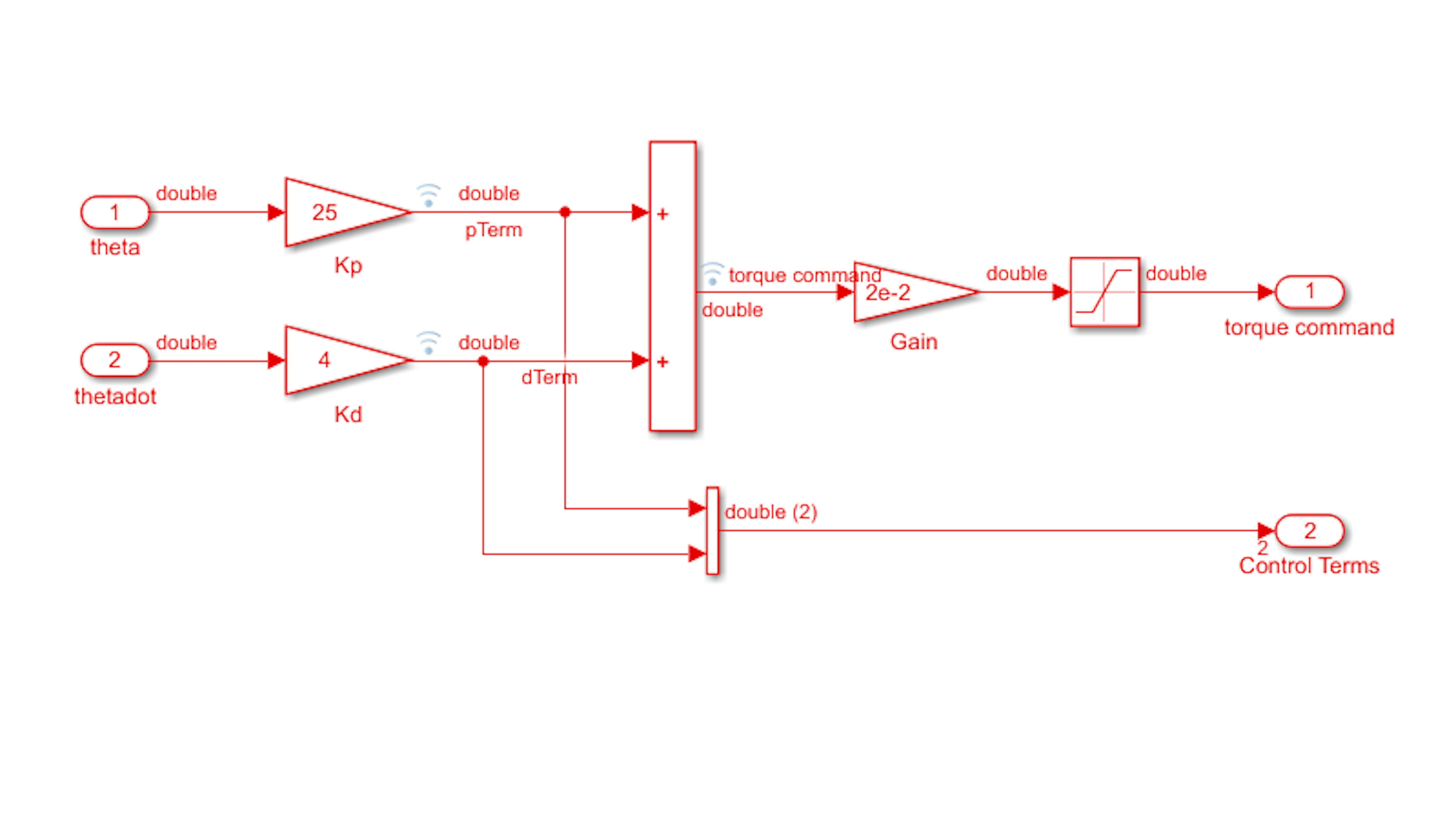
Access the Controller subsystem and edit the Gain block just before the outport to a gain value of 2e-2 (or 1.5e-2 for 6V motor). Change the signal and outport's name to torque command as shown below:
Note: The Kp and Kd have been divided by 2 to account for this increase in Gain value, so that we have the same controller that worked on the simulation model. For the 6 V motor, divide these values by 1.5.
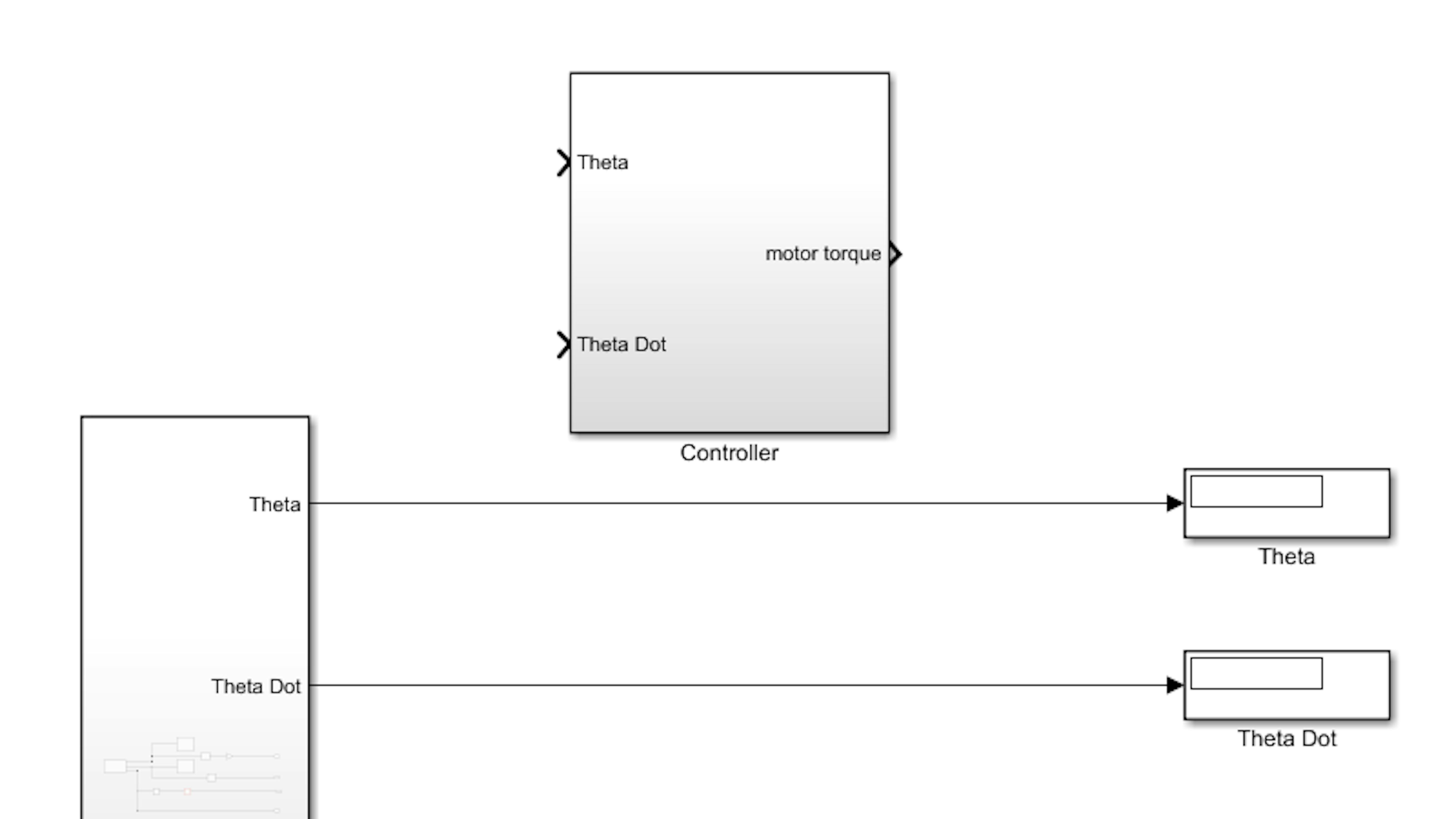
Delete the Theta and Theta Dot displays and name the signals as shown below. Connect these signals to the Controller as shown below:

Add a Scope block from Simulink → Sinks to this model. Branch and connect the theta signal, as shown:
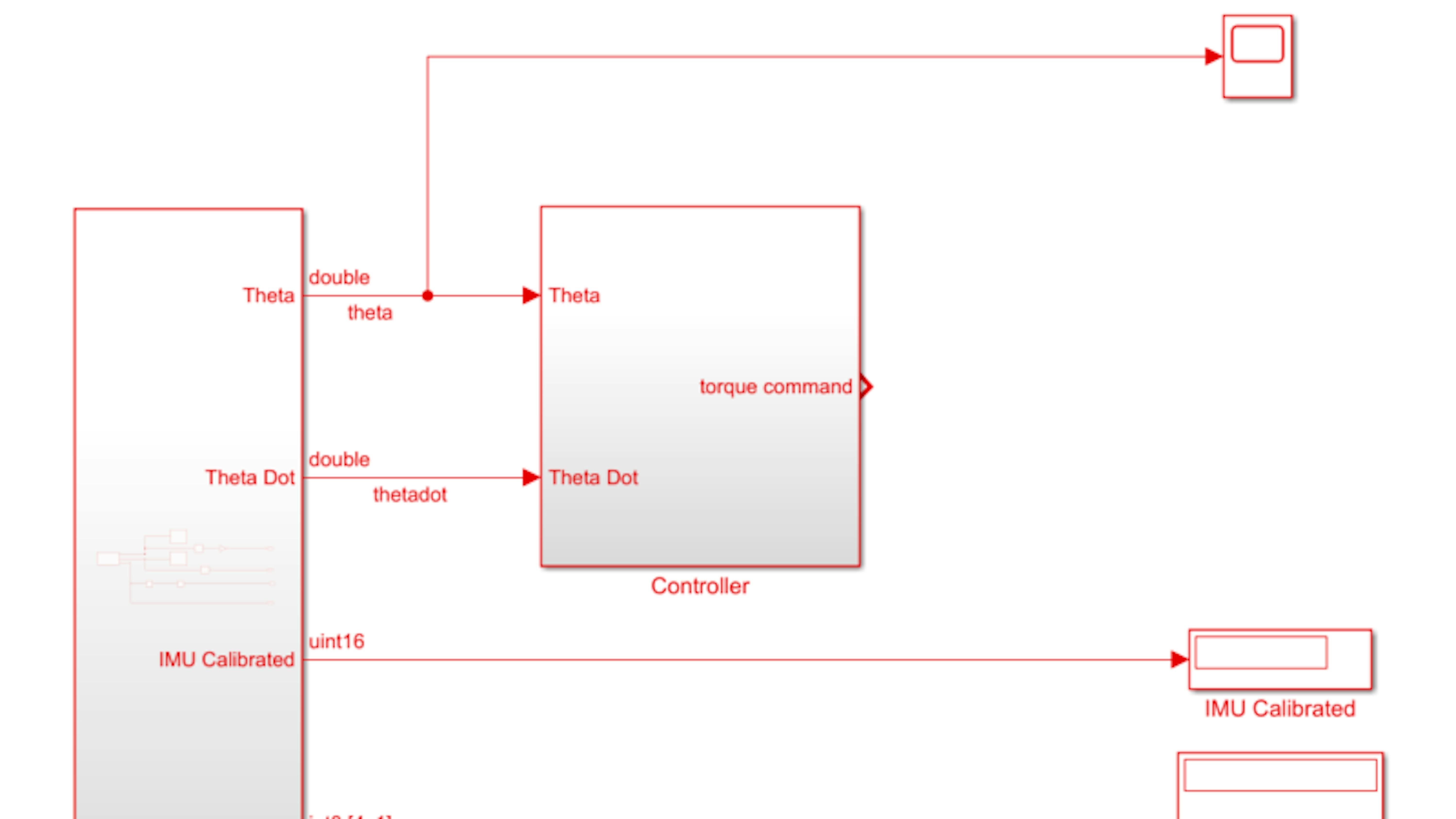
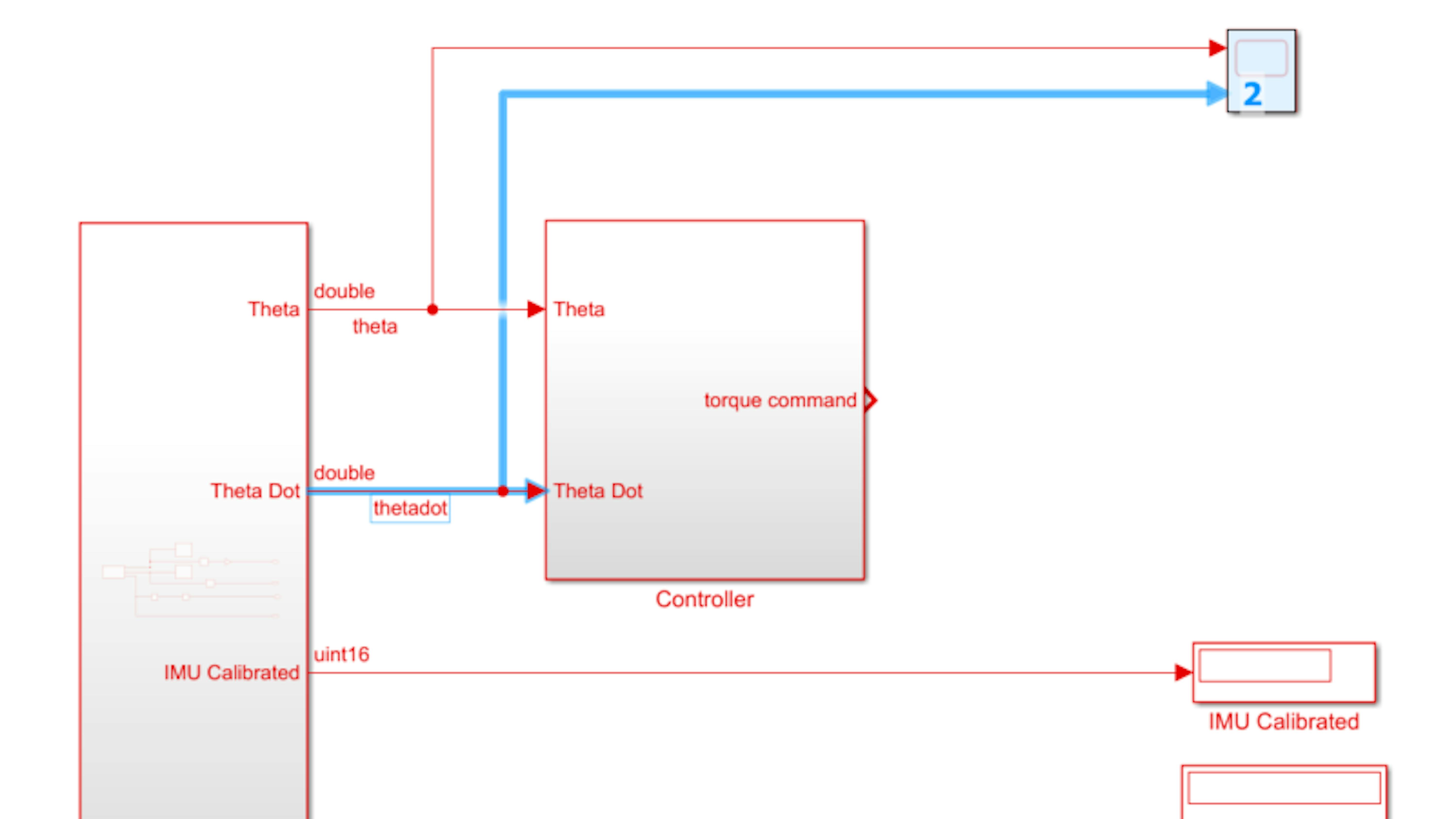
Now, right click on the thetadot signal to branch it and then drag the signal to the Scope block below the theta signal. A new inport will automatically form for you on the Scope block:
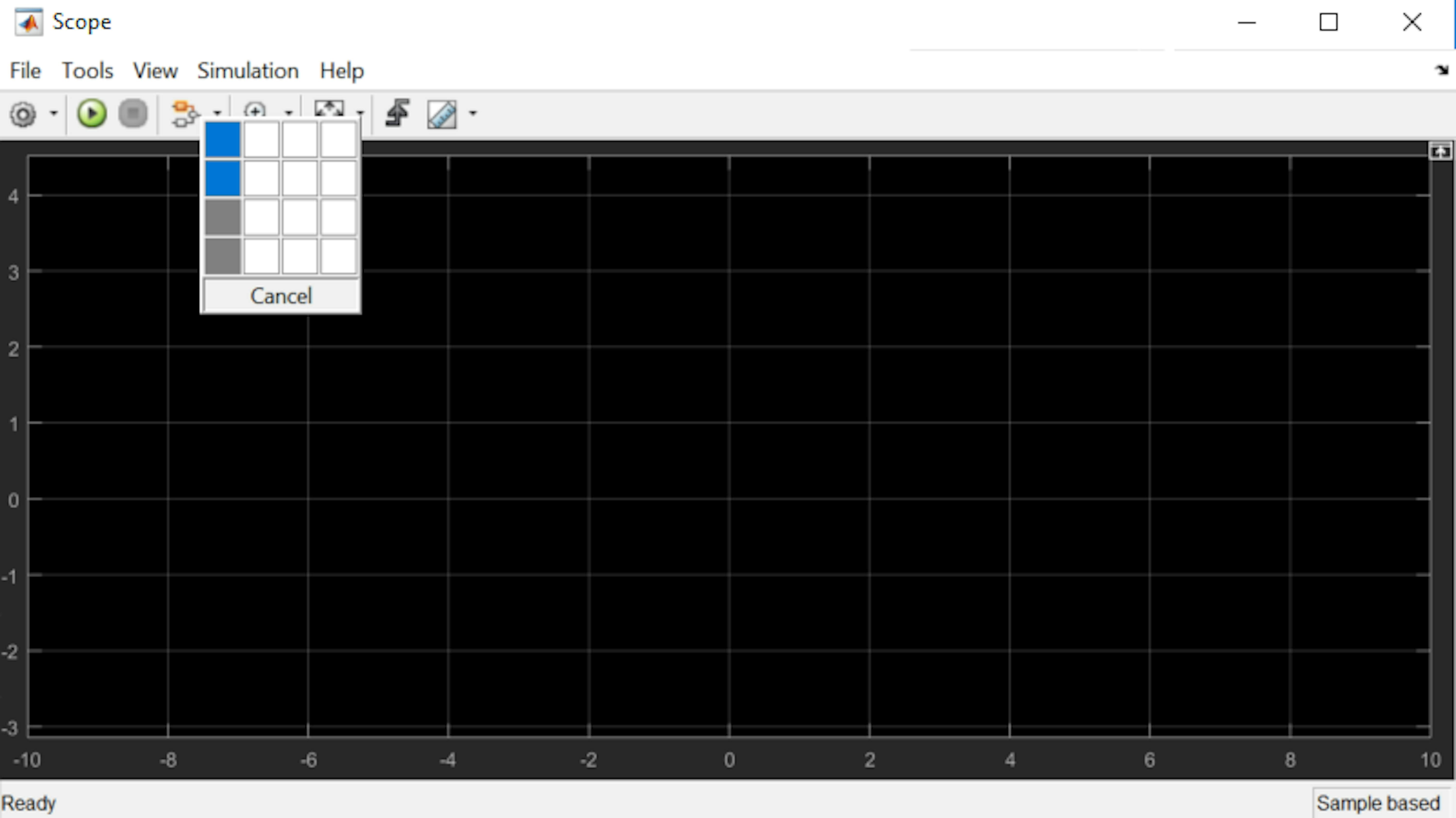
Next, configure the axes in the Scope block. In the Scope window, click View → Layout and set the layout to 4x1 (you will use the additional axes later):
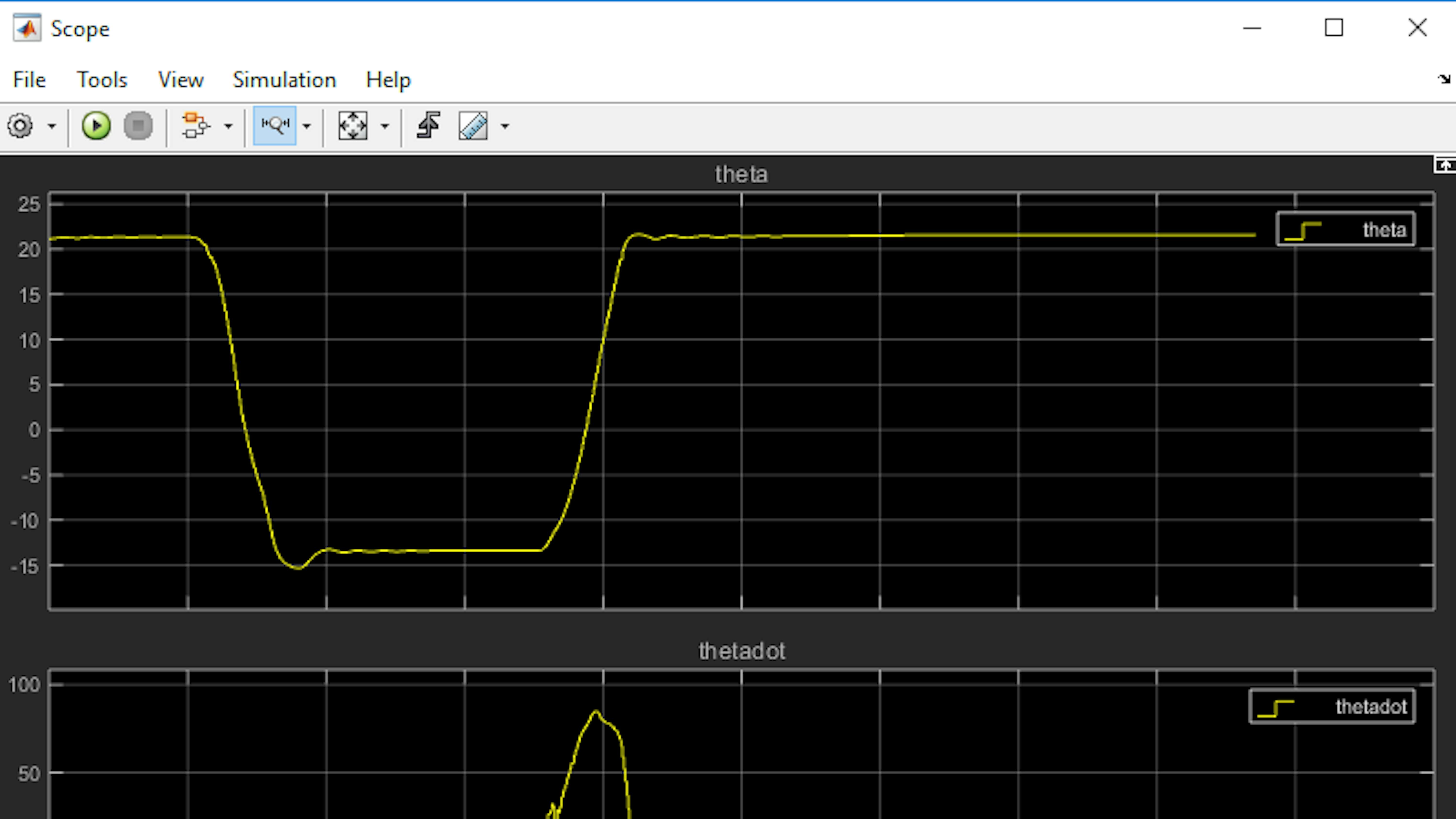
Run the model on the MKR1000 board and double click on the scope block to observe the Scope window. Try orienting the motorcycle about θ = 0, and revolving it several degrees in both directions:
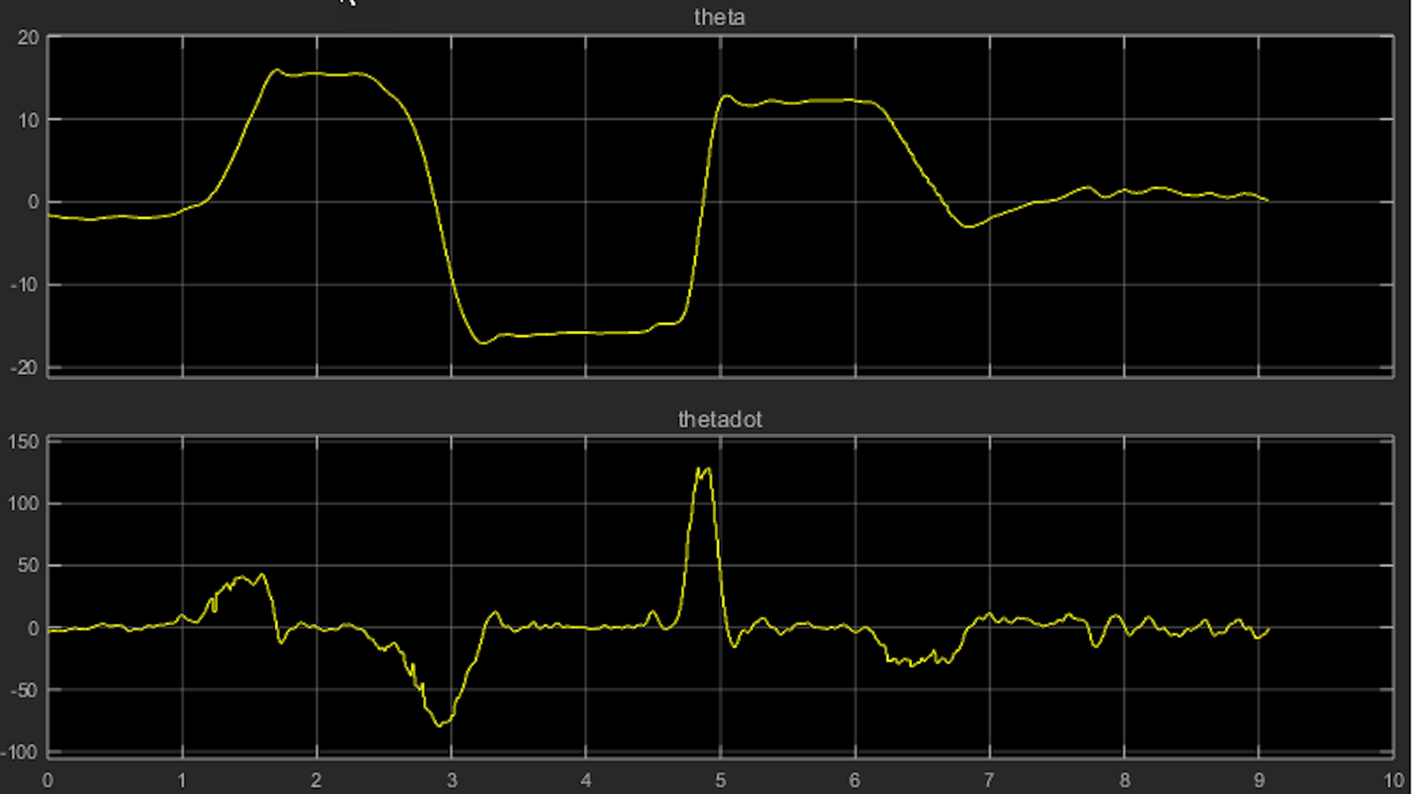
You can use the Scale Y-Axis Limits - press  button to rescale the vertical axes to fit the data.
Stop the model.
Next, let’s see how the controller algorithm responds to the IMU sensor data. Remember that the controller determines a torque command to send to the inertia wheel motor, based on θ and θ˙. You will want to observe the controller’s torque command signal along with θ and θ˙. Name the output signal from the controller as 'torque command' and then drag this signal into the bottom of the scope block. It will automatically provide a new inport numbered 3 as shown below:
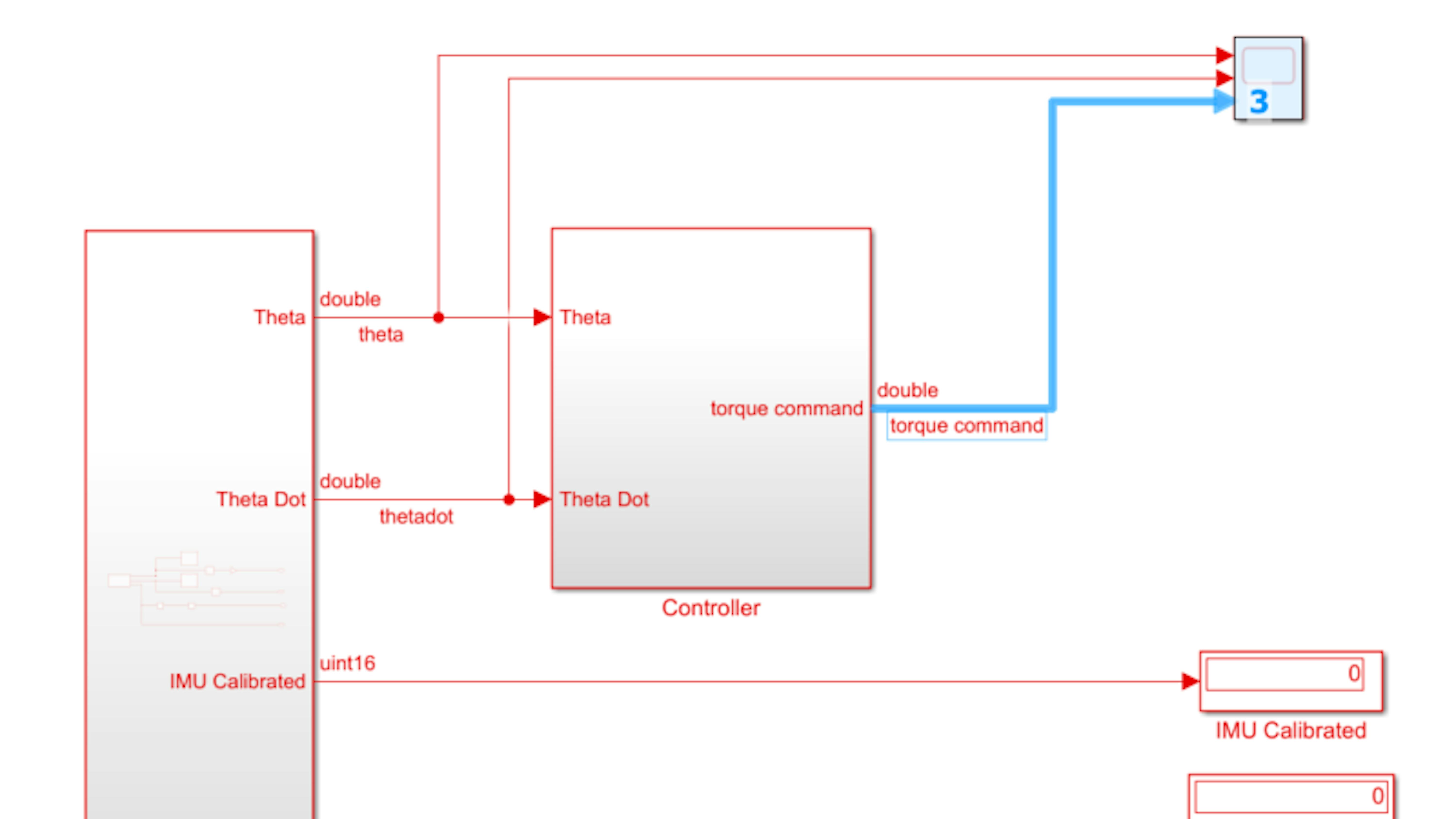
Run the model. Try holding the motorcycle as close to θ = 0 as you can while watching the torque command in the Scope window. Then, try leaning the motorcycle at small angles while observing the torque command:
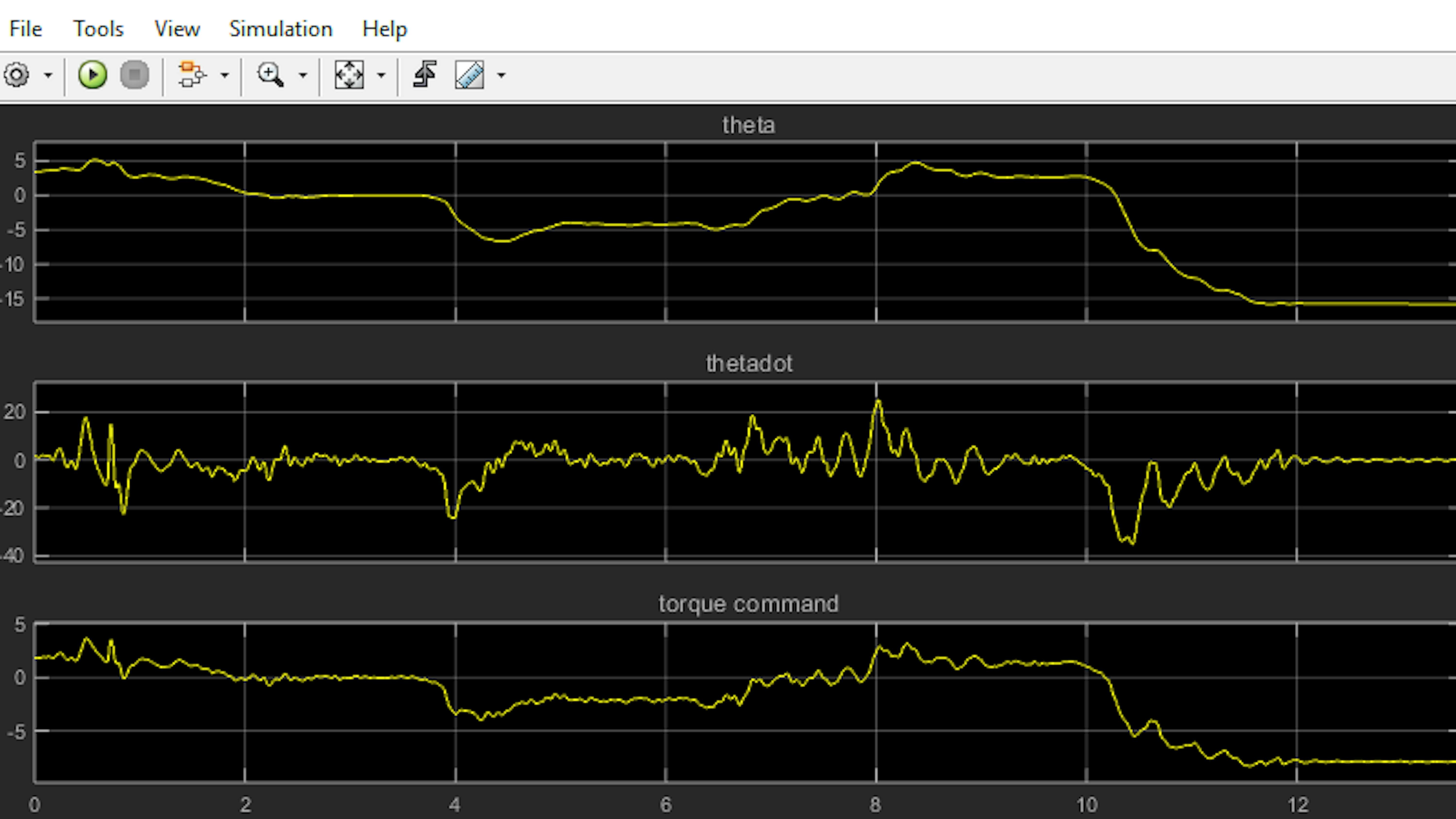
You should notice a few characteristic behaviors of the controller algorithm. First, when the motorcycle is held at a constant non-zero lean angle, the motor is generally commanded to generate torque in the same direction. This is consistent with what you should expect from the proportional term of the PD controller.
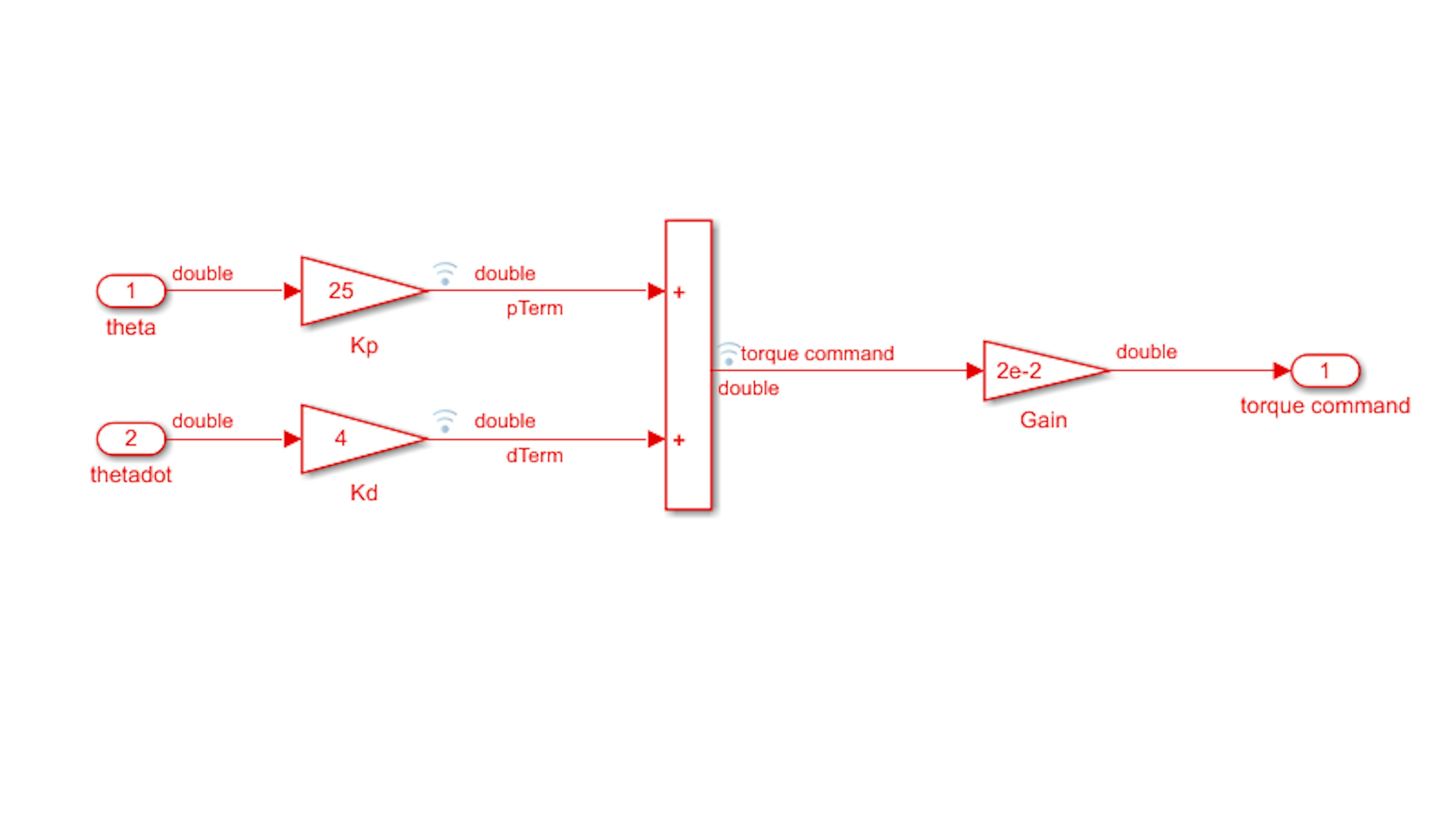
Stop the model and let’s take a look at how to better understand the relationship between the sensor information and the way the PD controller responds. To do so, you must monitor the P and D terms individually. To access these terms, go into the Controller subsystem and add a Mux block from Simulink → Signal Routing. Branch and connect the pTerm and dTerm signals to the Mux block, in this order.
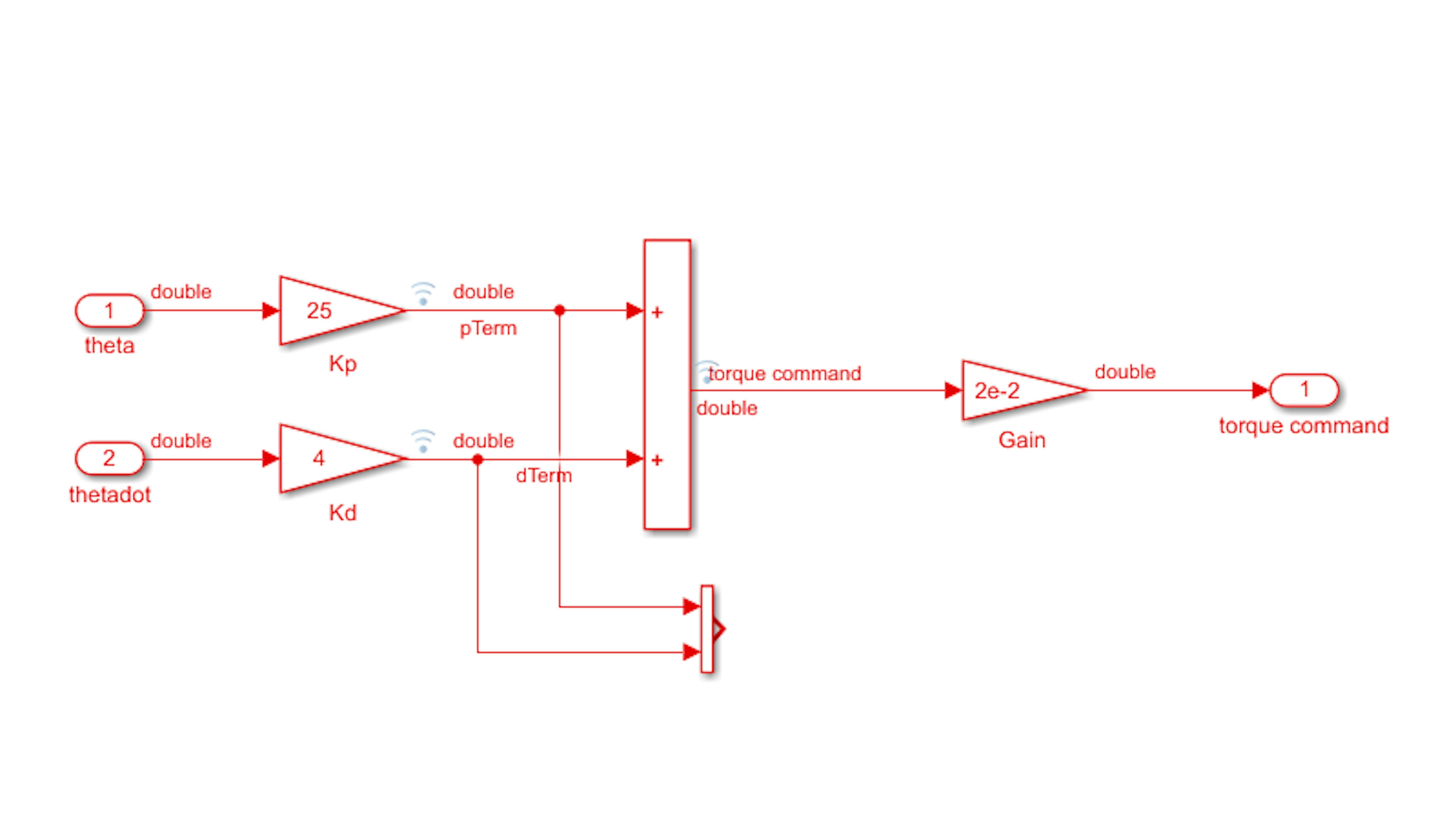
Now, add an Out1 block to export the PID terms. Connect and label the Out1 block as shown:
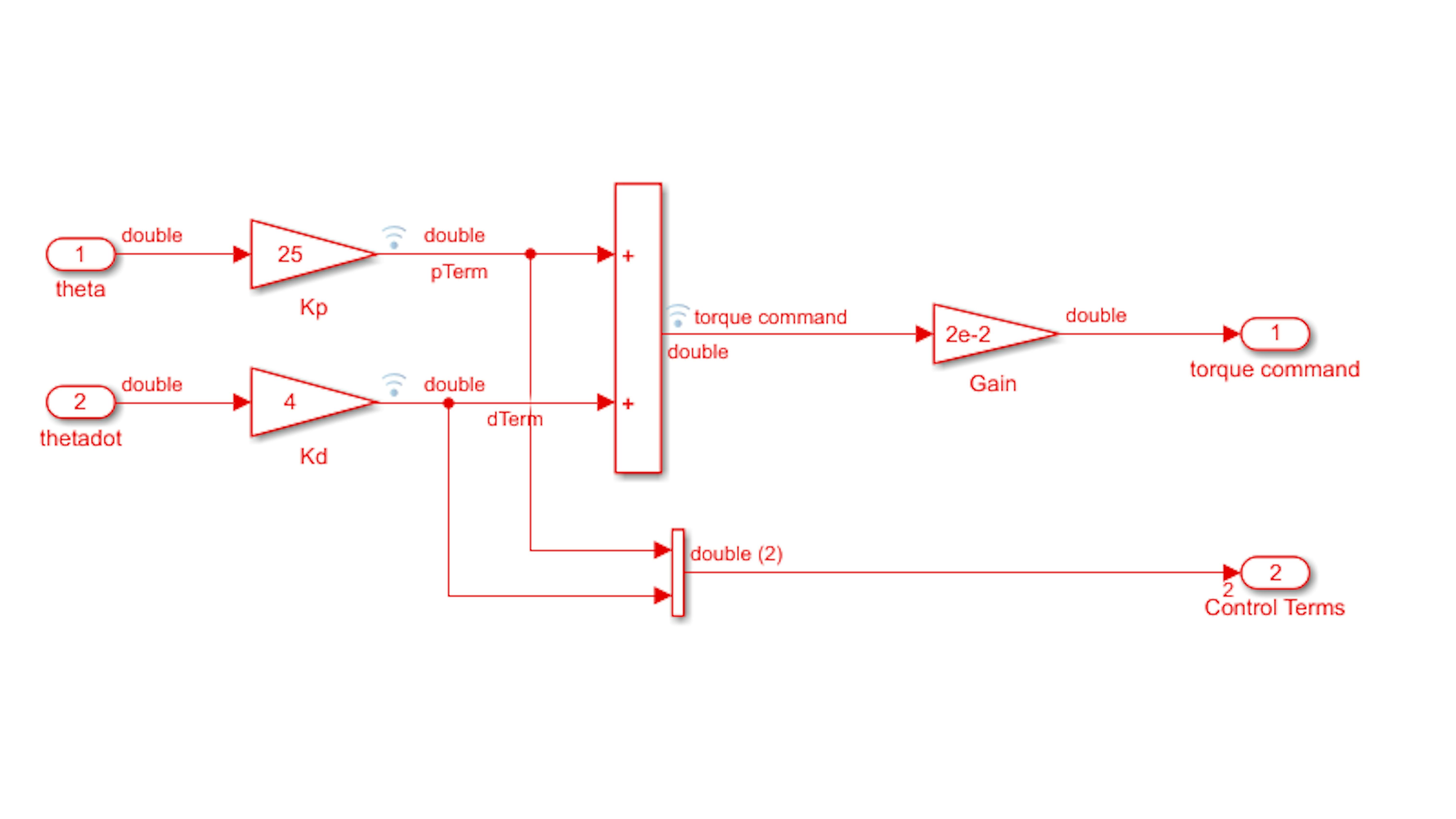
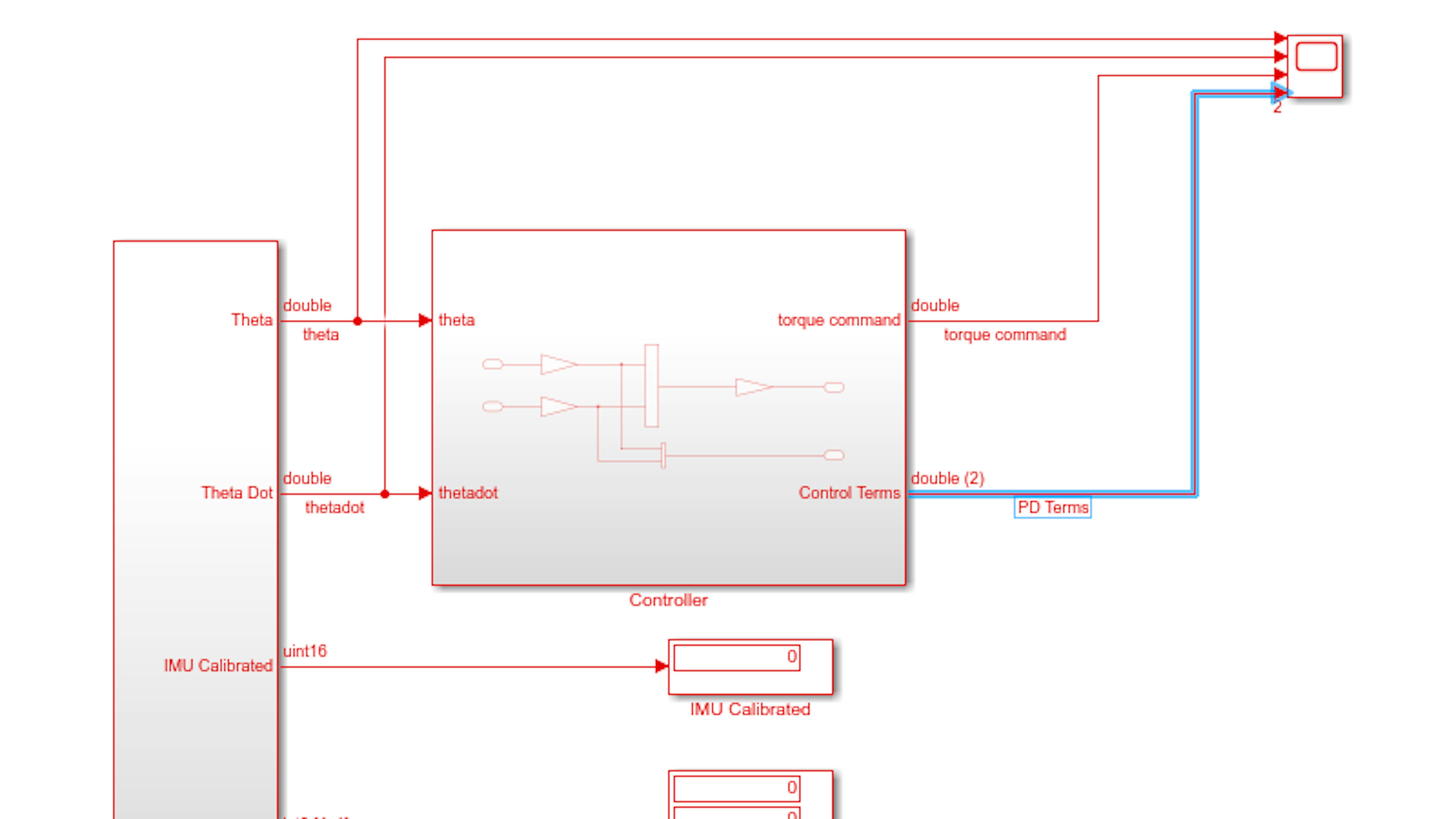
Return to the top level of the model, and route the Control Terms signal to the fourth position of the Scope block, as shown:
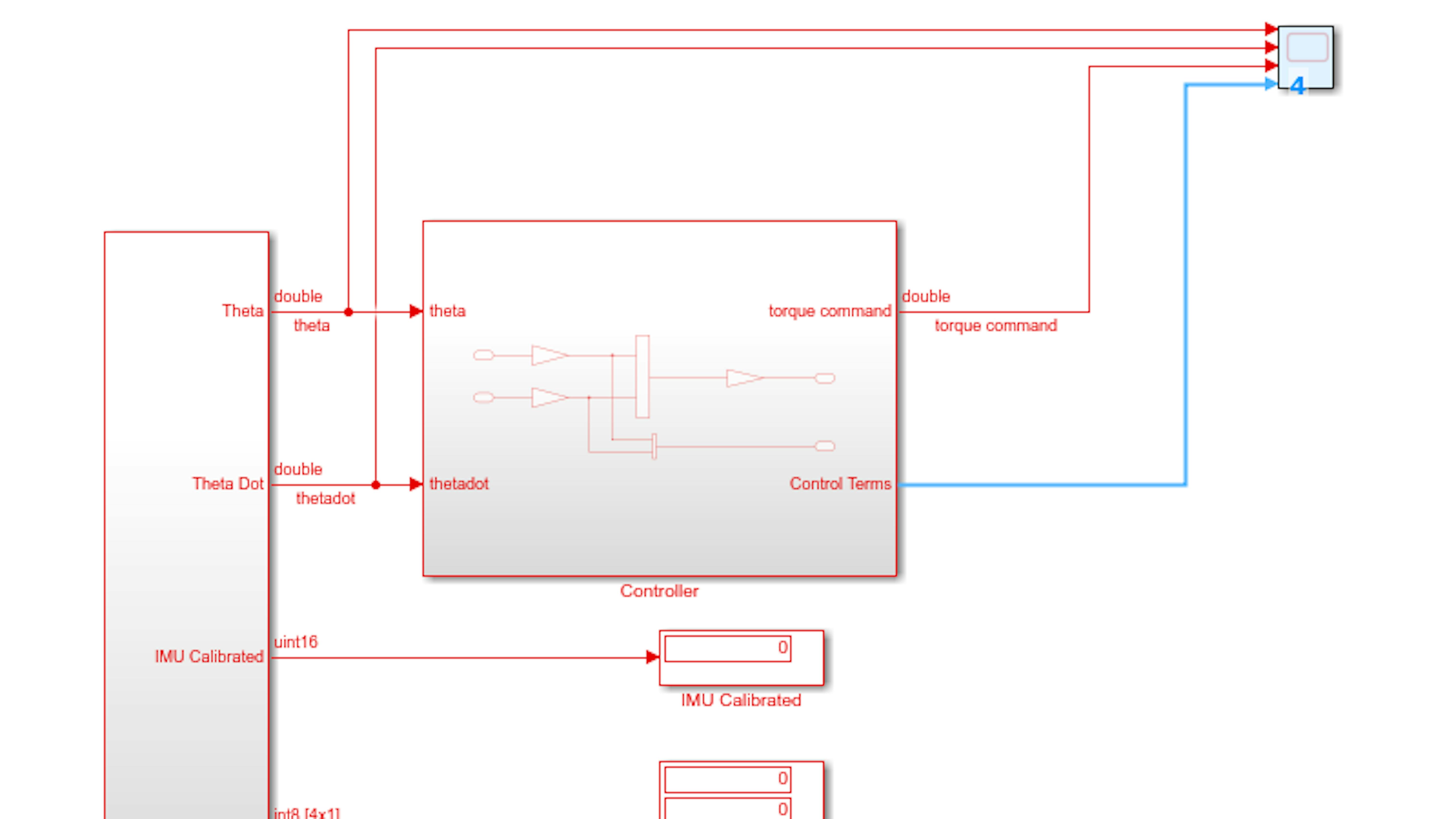
Label the new signal PD Terms:
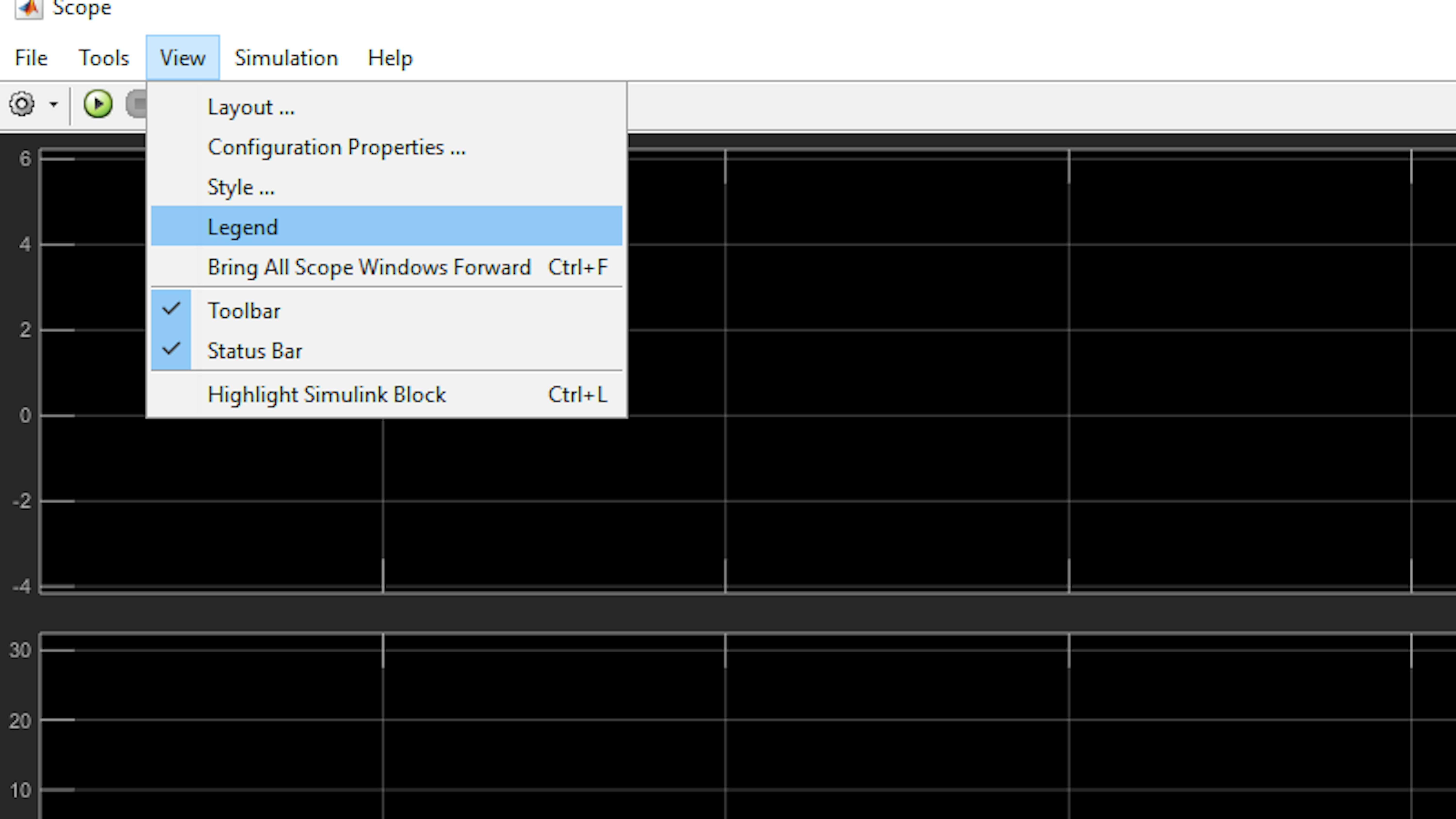
Inside the Scope window, enable the legend by clicking View → Legend:
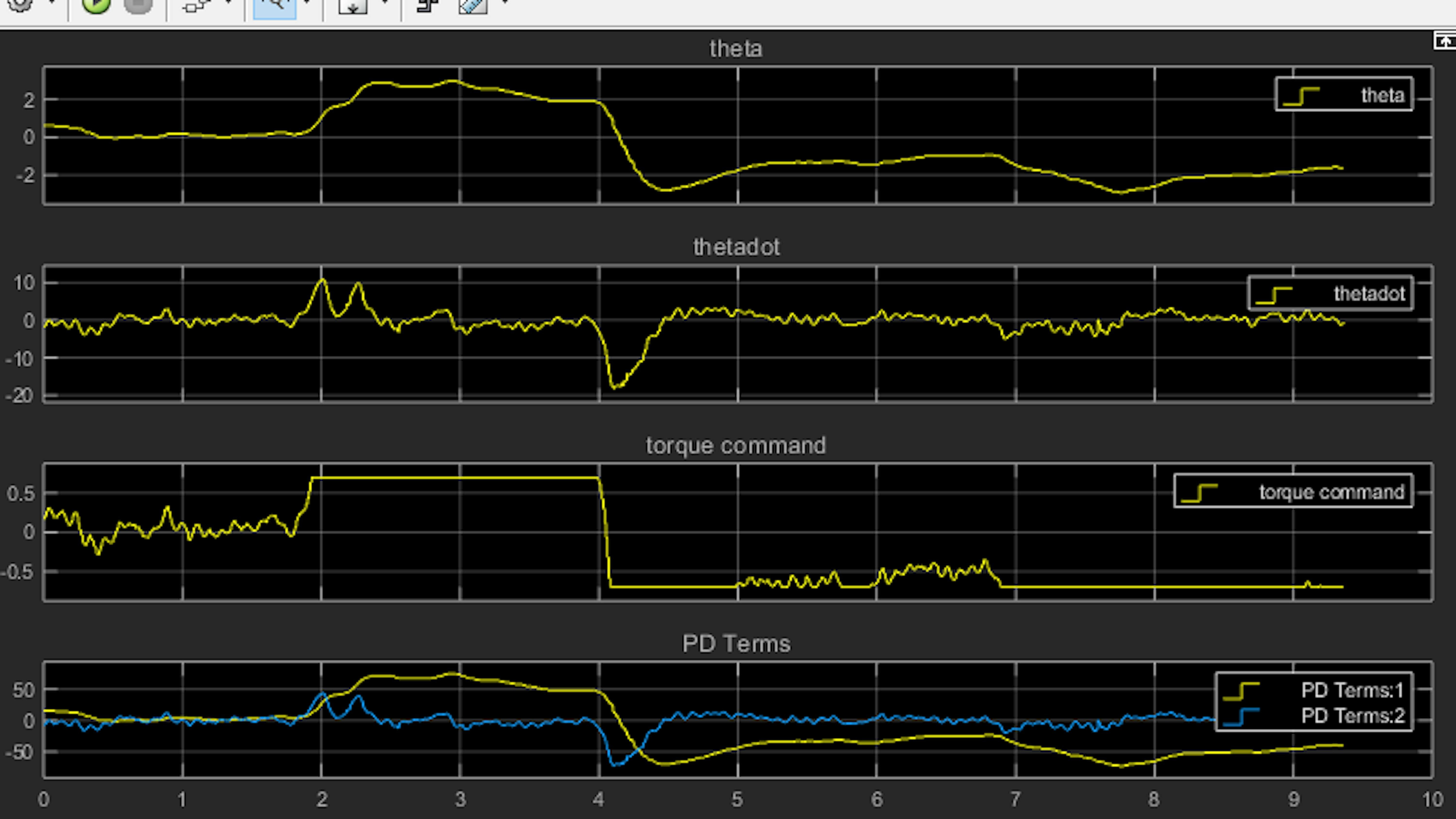
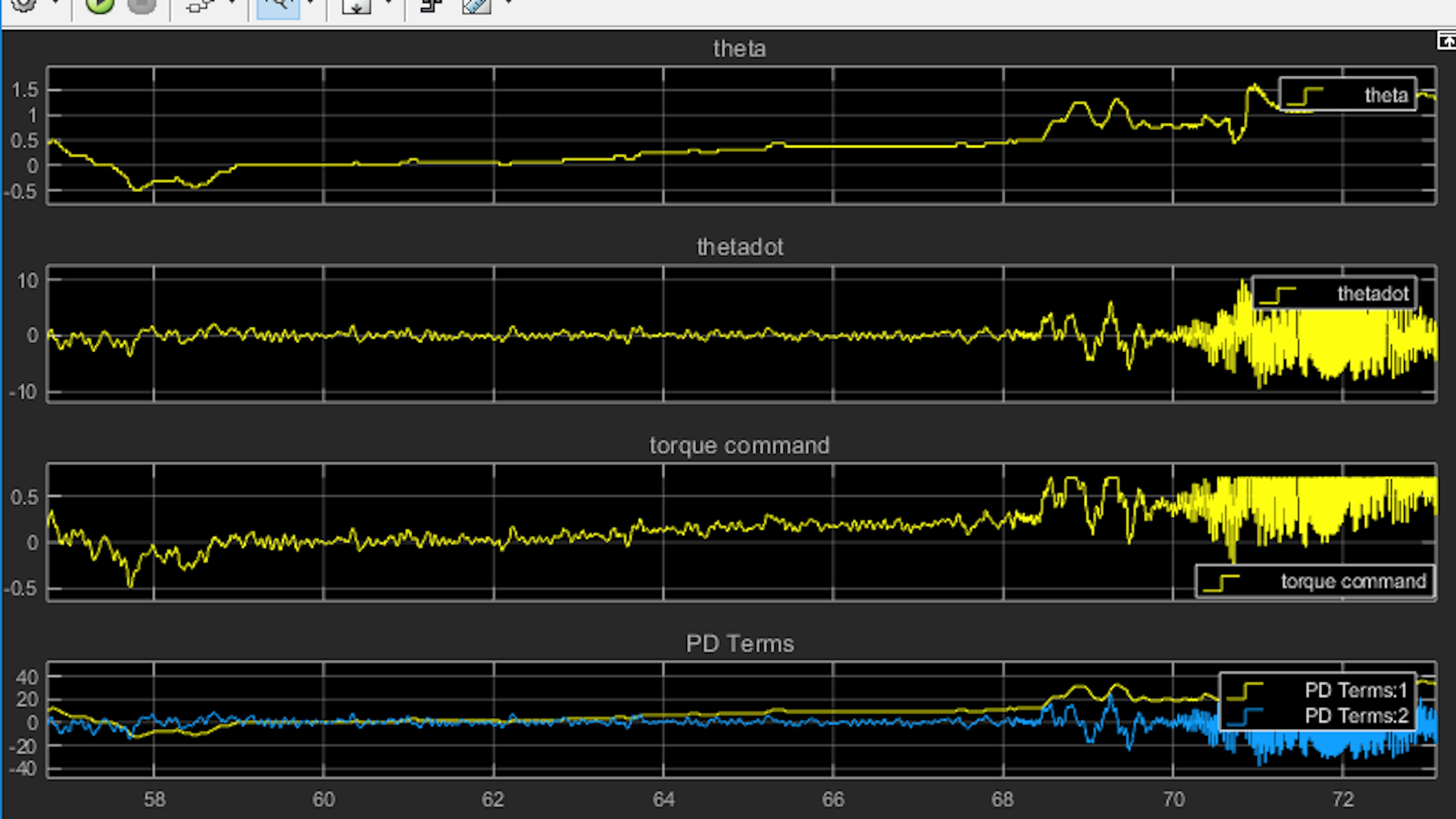
Run the model and examine the behavior of PD terms in the Scope window as you adjust the lean angle:
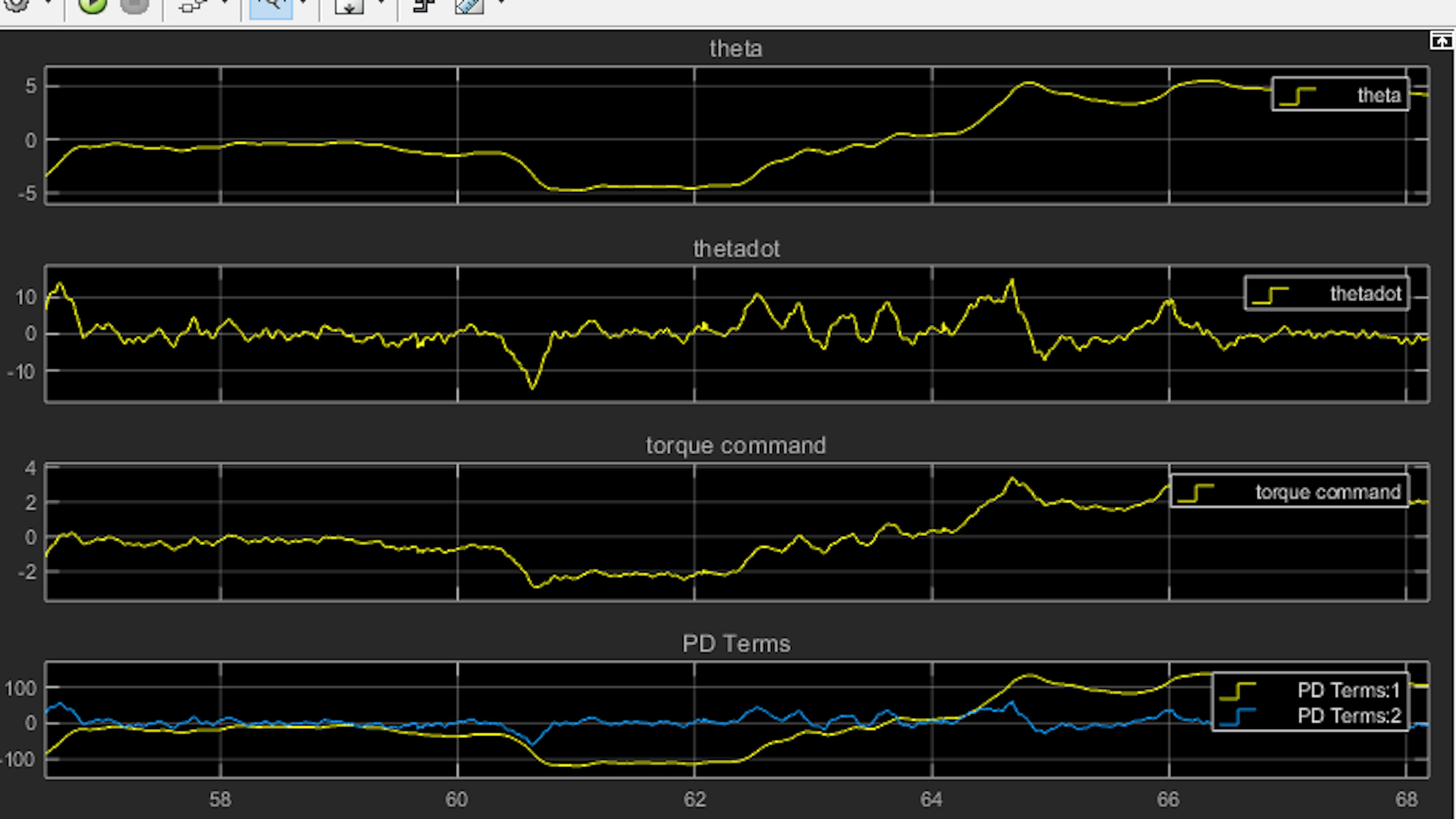
Here P is PD terms: 1 and D is PD terms: 2. Even if your signals do not look exactly the same, you should observe that the proportional (P) term has the same shape as theta (but a different amplitude) and the differential term is smaller in magnitude compared to P term. This is a good rule of thumb, the P term should generally dominate the torque command, while the I and D terms merely augment the proportional response (in our case just the D term).
Next, have a look at the torque command in the Scope window. Earlier, we discussed that the torque command must operationally run from -0.7 to 0.7. As you can see, the controller is currently commanding torque well outside this range. To ensure that the controller does not command an impossible torque, you must saturate the torque command.
Press the stop button on the model. Add a Saturation block to the Controller subsystem (Simulink → Discontinuities). Place it immediately before the Torque Command outport block and set the saturation limits to 0.7 and -0.7:
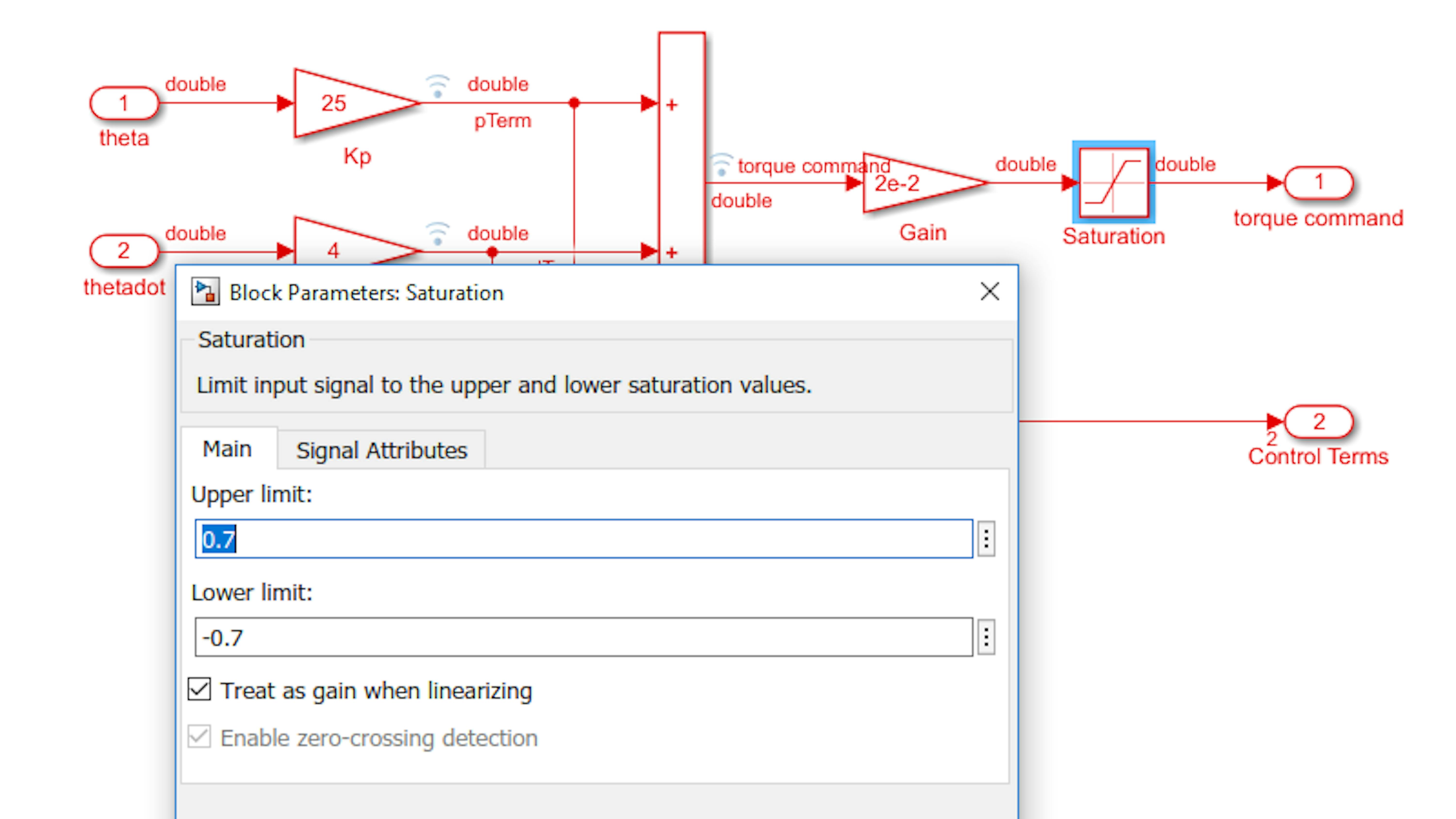
Run the model and observe the torque command in the Scope window while varying the lean angle around a few degrees around θ = 0 (within +/- 4):
You will see that the torque command is spending a large fraction of the time at the limits of the saturation condition. You generally want the torque command to saturate very rarely because it can damage the motor and surrounding hardware if it persists for too long. That is why, we are carefully assessing the controller behavior before connecting the inertia wheel DC motor! It is also not good for balance since saturation makes it impossible for the motor torque to respond to variations in θ and θ˙. This is where the Inertia wheel models that we worked on in the last exercise will come in handy.
Stop the model if it is still running and Open myIWheel.slx:
>> myIWheelNote: If myIWheel.slx is unavailable or incomplete, use iWheel2_tach.slx instead
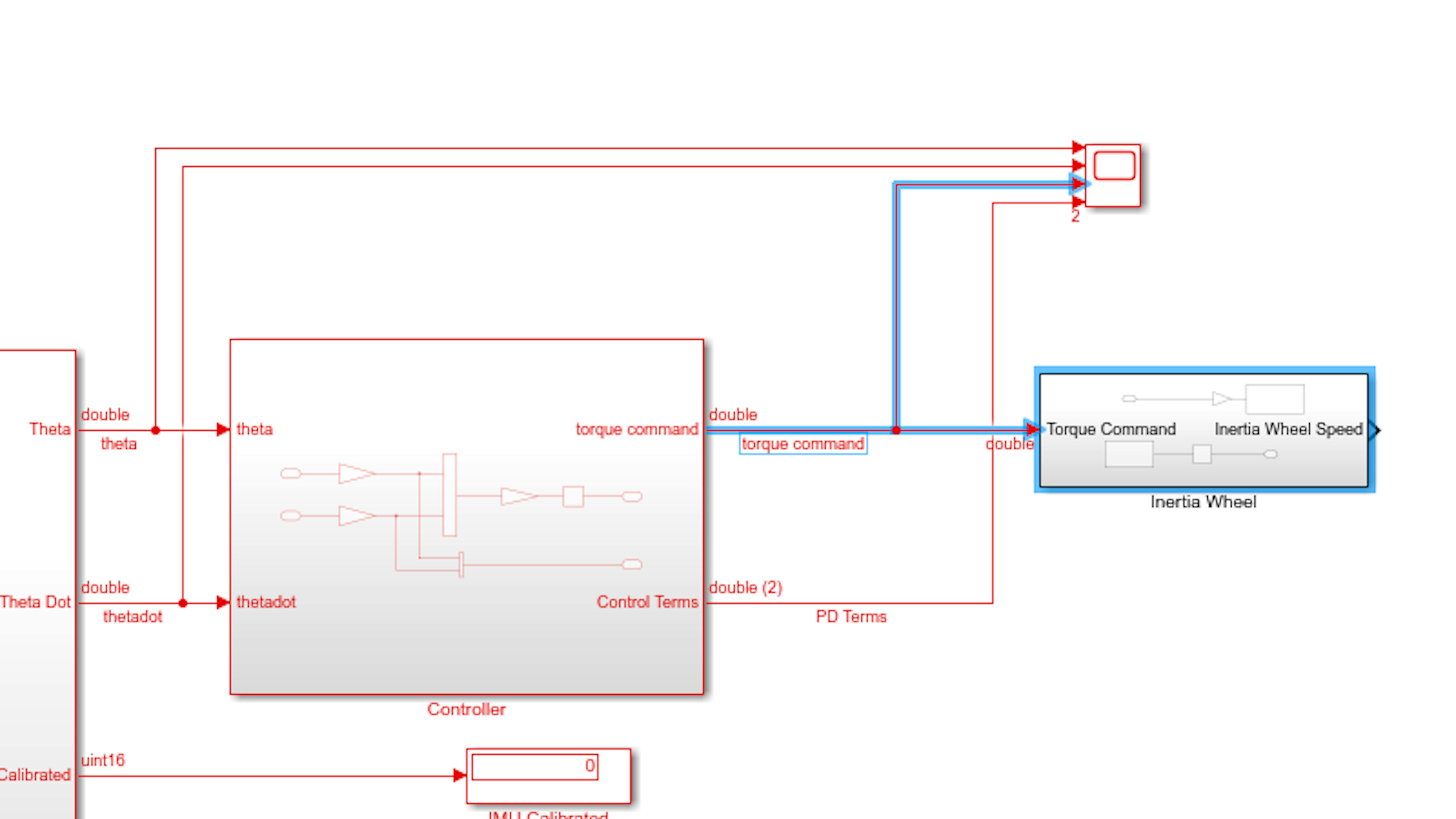
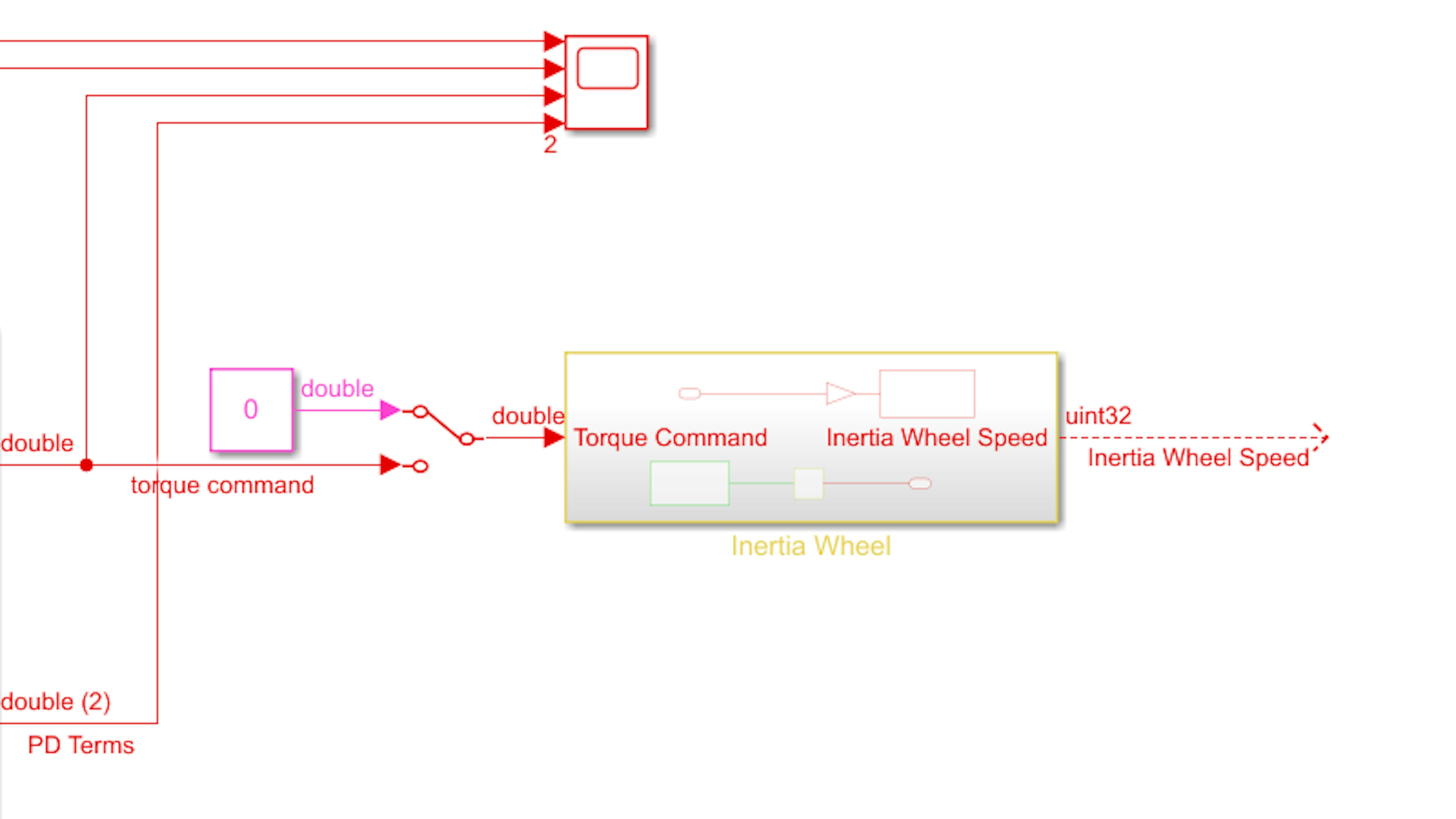
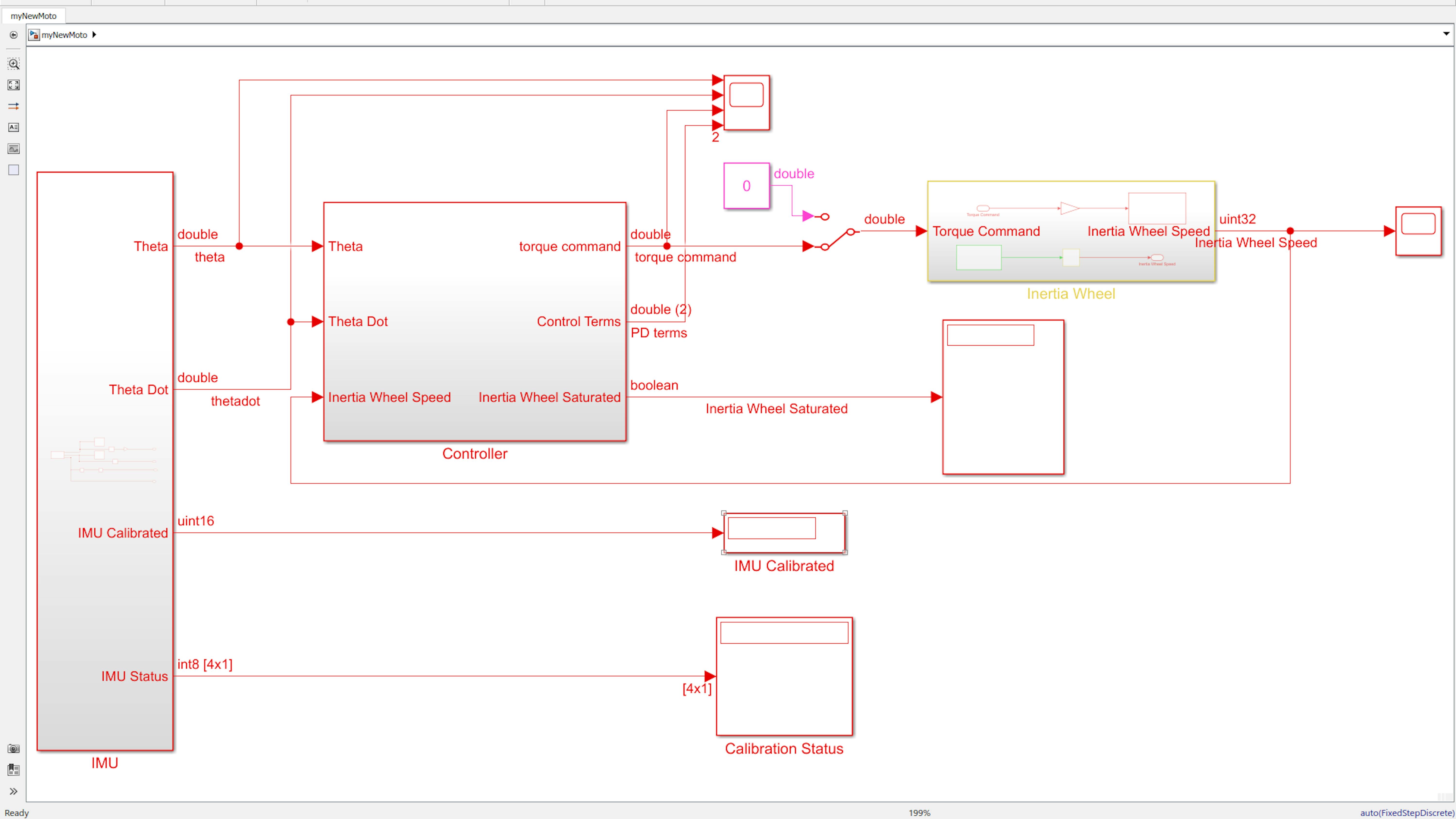
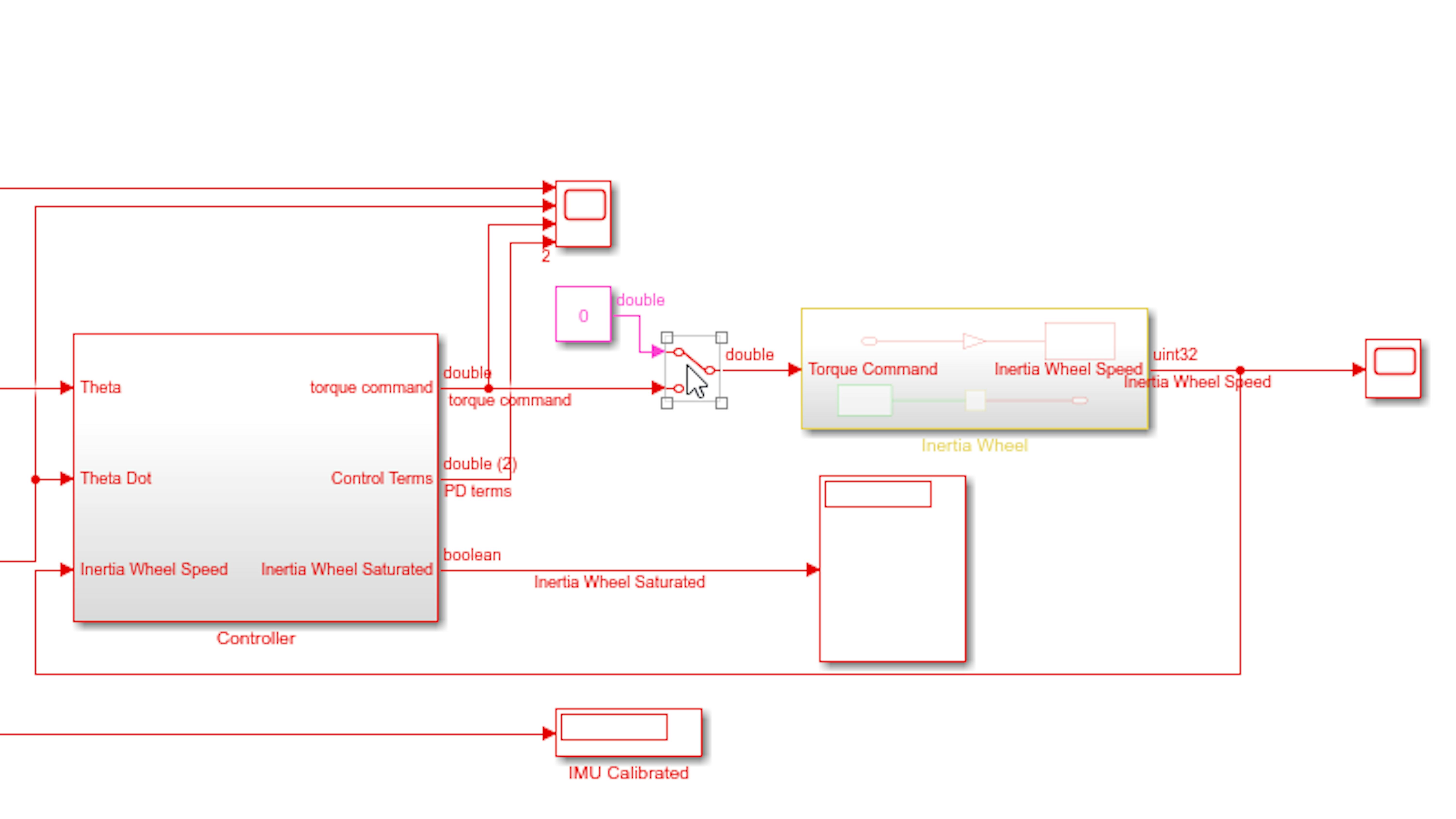
Copy the Inertia Wheel subsystem from myIWheel.slx to myNewMoto.slx and connect it to the “torque command” signal as shown:
It would be ideal to switch the Inertia wheel ON and OFF as needed. Let’s see how to add a switch to the model so that you can enable or disable the inertia wheel motor at any time from Simulink. This is useful if you want to calibrate the IMU before attempting to balance the motorcycle or if the inertia wheel picks up too much speed. Add a Manual Switch (from Simulink → Signal Routing) block to the top level of the model and route the signals as follows:
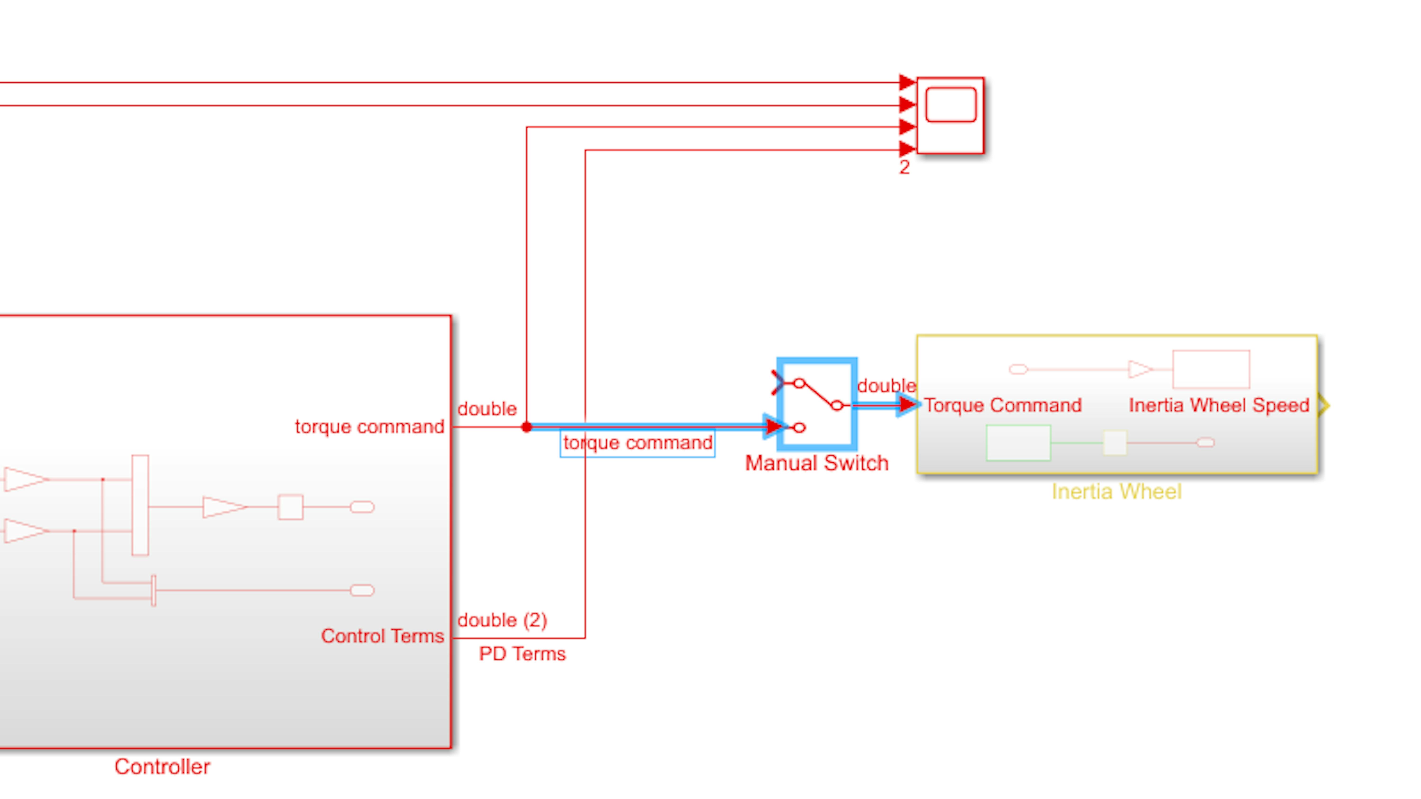
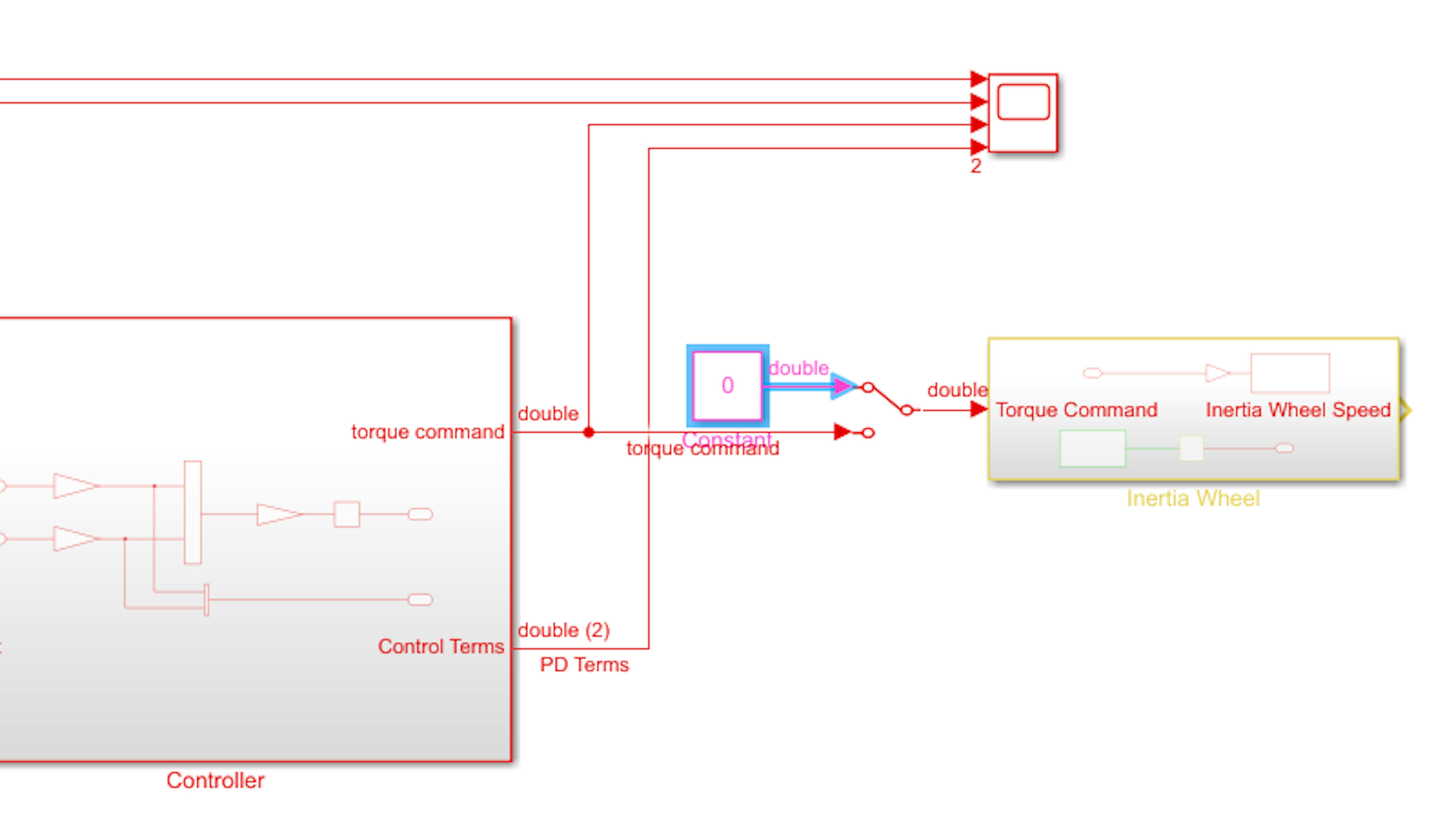
Add a Constant block from Simulink → Sources and set the constant value to 0. Double-click the Manual Switch block to point the Inertia Wheel signal source to 0:
At this point, you do not necessarily expect the motorcycle to balance stably (it may be marginally stable), but you should see the inertia wheel respond to the lean angle direction.
Please read and follow the instructions before running the model:
- Ensure that the Gain inside the Controller subsystem is set to 2e-2.
- In the Controller subsystem, set the PD gains as follows:
Kp = 25
Kd = 4
- Run the model with the inertia wheel disabled (manual switch toward 0).
- Open the Scope window when the application starts running.
- Make sure that the IMU is calibrated, if not spin the motorcycle along all three principal axes.
- Hold the motorcycle close to the vertical plane so that you see the theta signal close to zero in the scope.
- Adjust the lean angle until the torque command signal approaches zero as well. Then, enable the inertia wheel motor while holding the motorcycle by double clicking on the manual switch.
- Try leaning the motorcycle a few degrees left and right. The inertia wheel should accelerate in the same direction as the motorcycle is leaning.
- Try releasing the motorcycle at θ = 0. See if you get any degree of balance (it is okay if it does not balance right now, but you may be surprised!).
- When you are finished, disable the inertia wheel motor (by double clicking on the manual switch), and stop the model.
Note: If the inertia wheel starts to pick up too much speed, be prepared to double-click the manual switch in the model or flip the power switch on the motor carrier to OFF.
Regardless of whether you achieve marginal balance, you should observe that the inertia wheel accelerates in the same direction as the lean angle. With the drive gain set low, you should see that the torque command rarely, if ever, reaches the saturation limits at 0.7 and -0.7 when the lean angle is close to zero. When the lean angle is a high value (greater than +/-3 degrees), it makes sense that the torque command is at +/- 0.7 and still the motorcycle cannot reverse its direction. .
When oscillations occur about θ = 0, notice the similar oscillatory frequency of the P and D terms (see screenshot above if you did not observe such oscillations). A useful way to think about a PID control is as follows: the proportional term is correcting for the error being observed right now, the integral term is correcting for the errors of the recent past, and the derivative term is correcting for errors that are projected to occur in the near future. This explains why D term peaks occur before those of the proportional term.
Stop the model if you haven’t already. Feel the inertia wheel motor with your fingers. Is it hot?When you run the DC motor at high torque commands for several minutes, large currents are drawn, and a lot of heat is generated. As you are building your system model and testing it on the MKR1000 and the motorcycle hardware, you should frequently (i.e. every few minutes) feel the inertia wheel motor to make sure it is not overheating. As described earlier, any motor can become permanently damaged if it gets too hot for too long. Additionally, the Motor Carrier can become damaged from having so much current drawn in a short period of time. While the Motor Carrier comes with firmware that automatically shuts down the motor leads under certain dangerous conditions, you should not rely on that completely to safeguard the Motor Carrier. Safety should be part of your algorithm!
IMPORTANT: When your inertia wheel motor becomes uncomfortably hot to the touch, disable the inertia wheel motor in the model, stop the model, power off the motor carrier, remove the battery, and let the system cool for at least 15 minutes.
Following the above rule is the surest way to prevent having to buy a new DC motor or motor carrier.
In the following section, you will add some safety mechanisms to the controller algorithm that will make it very unlikely (but still possible) that hardware damage will occur. After those safety features are added, you will refine your balance control algorithm, which will require lengthy model runs with the inertia wheel motor enabled.
ADDING FAILSAFE FEATURES
You now have a controller that accelerates the inertia wheel in the correct direction according to the sign of the lean angle. You added a manual switch to the inertia wheel so that you can shut it off before and after balancing and when abnormal conditions arise, such as the inertia wheel spinning too fast or the motorcycle falling over. To make the controller robust and autonomous, let’s add some safety features to the controller algorithm to shut off the inertia wheel automatically under the following conditions:
-
Inertia wheel spins too fast (risk of damaging motor)
-
Motorcycle “falls” outside a range of “normal” lean angles (risk of damaging inertia wheel or ground surface)
- IMU is not calibrated (risk of destabilizing controller due to inaccurate set point)
- Battery is undercharged
Inertia wheel spinning too fast
First, let’s add a mechanism to automatically shut off the inertia wheel motor if it spins too fast. Recall that in the previous exercise, you used the tachometer to measure the inertia wheel’s angular speed and implemented some logic to shut off the inertia wheel motor when a speed threshold is exceeded. The balance control algorithm should do the same thing.
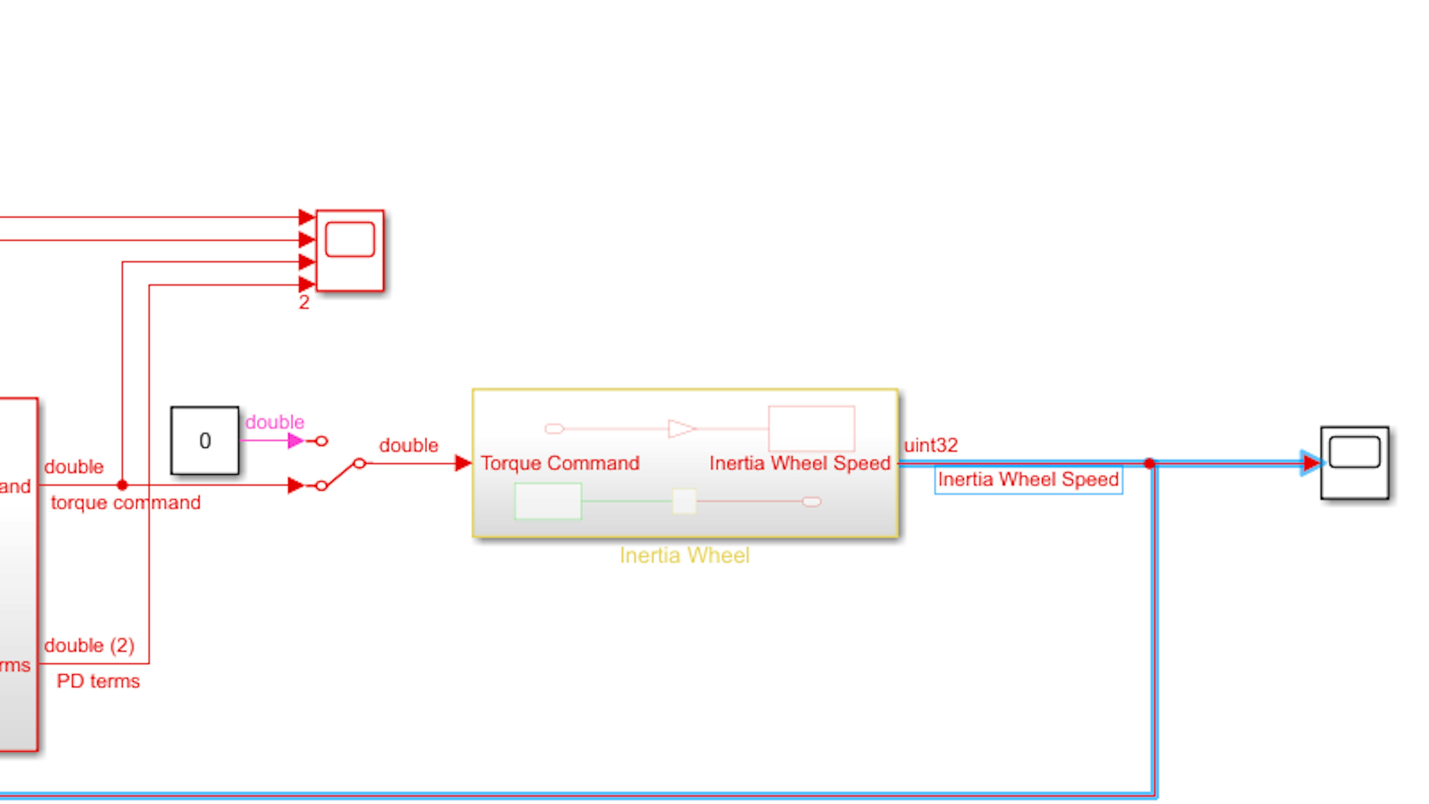
Label the output signal from the Inertia Wheel subsystem outport as Inertia Wheel Speed:
Now drag the signal into the left side of the Controller subsystem, creating a third inport:
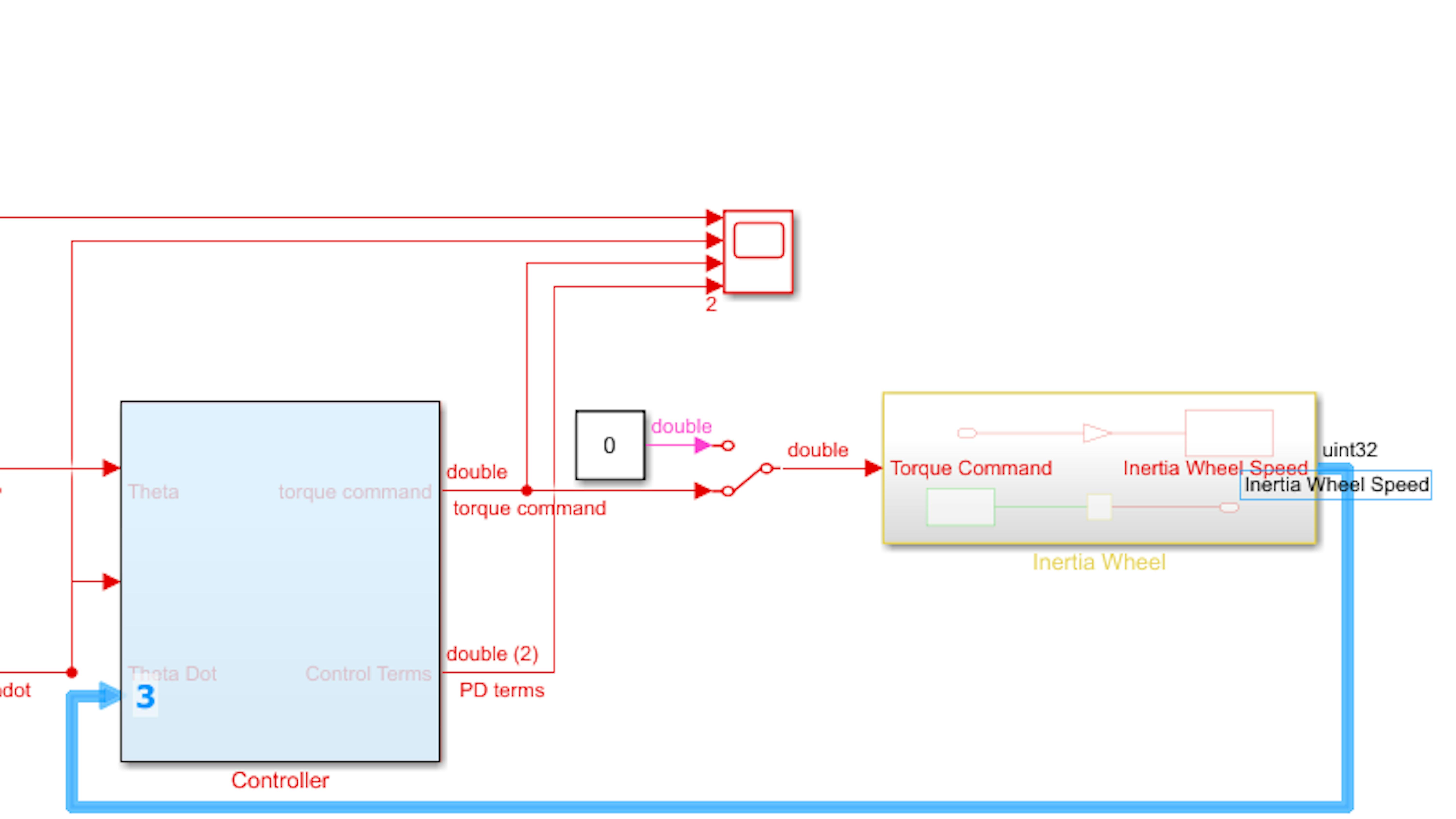
Branch the signal into a new Scope block (Simulink → Sinks). Open the scope block and change View → Layout to 3x1:
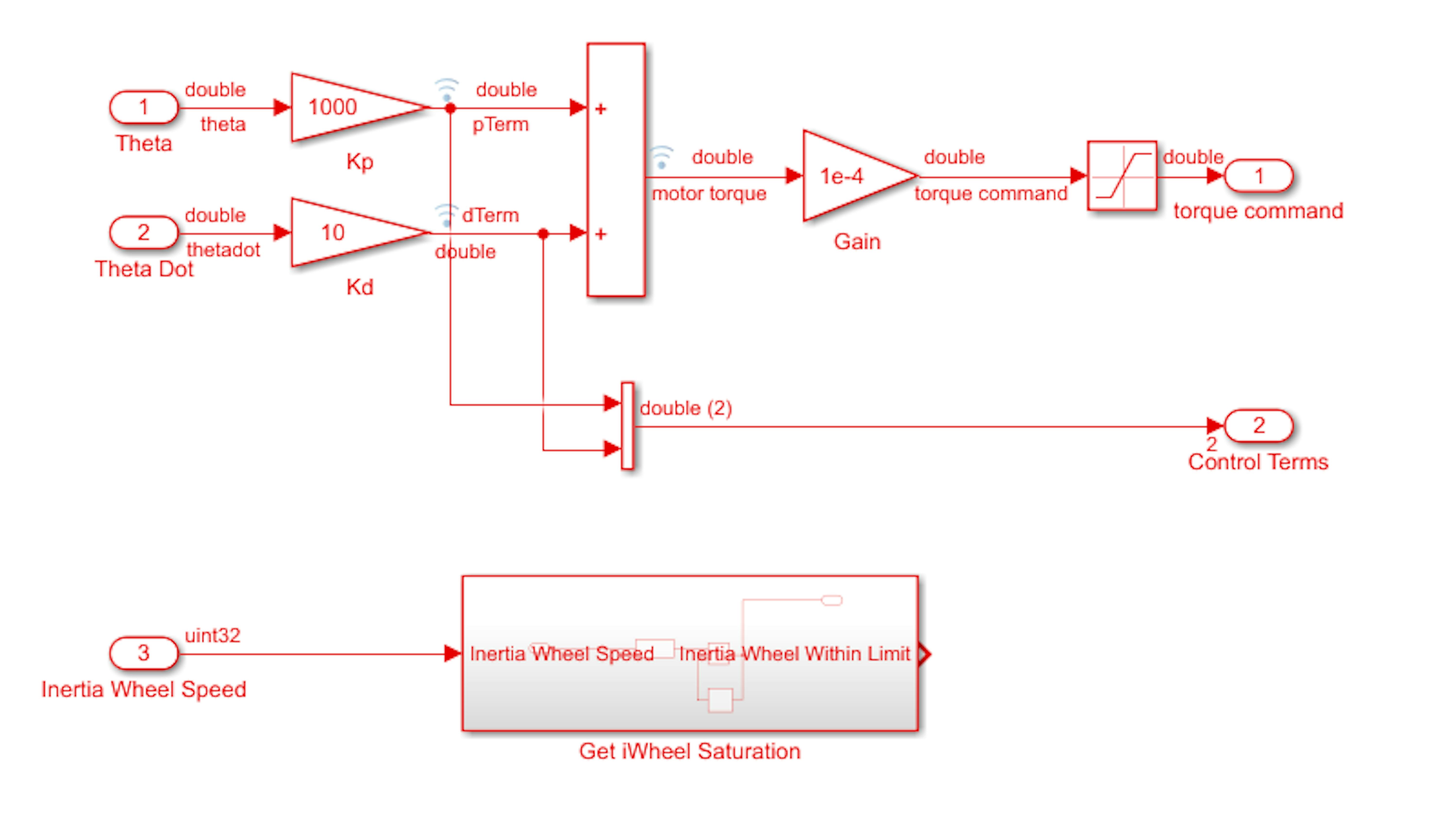
Next, go to myIWheel.slx (or iWheel2_tach.slx), copy the Get iWheel Saturation subsystem, and paste it into the Controller subsystem in myNewMoto.slx. Route the signals as shown:
Note: Compare to Constant value will change when tachometer becomes available.
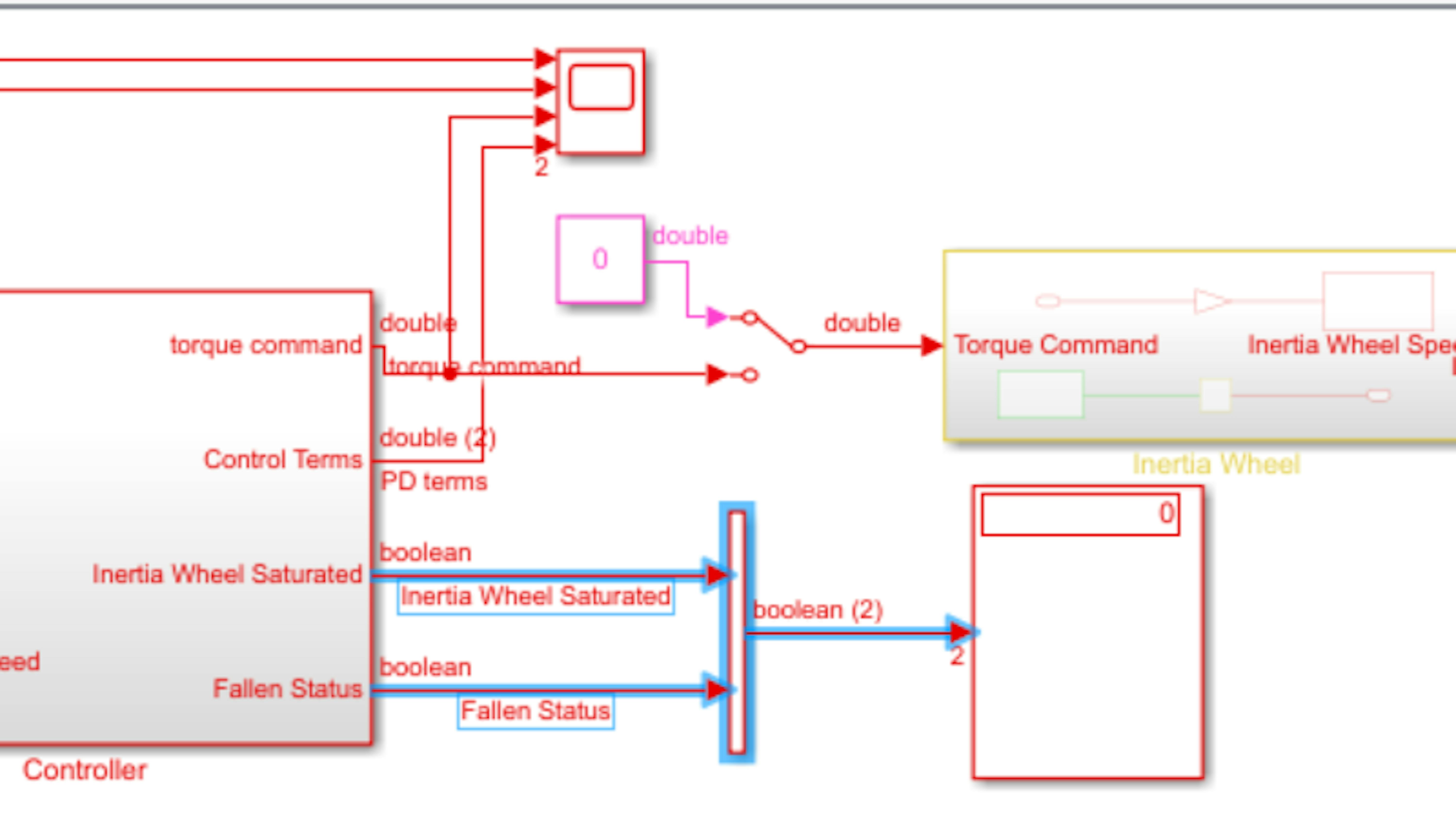
The output of the Get iWheel Saturation subsystem is a logical value of 0 or 1. When the value is 1, the inertia wheel motor should operate according to the controller output. When the value is 0, the inertia wheel motor should stop. In other words, the ultimate torque command should be the product of the controller output and the subsystem output. To implement inertia wheel saturation shutoff, add a Product block from Simulink → Math Operations and route the signals as shown:
Now, hold the motorcycle in the vertical position and run the model on the MKR1000 board. Enable the inertia wheel and as lean the motorcycle in one direction to say 3 degrees and hold it there. You will see that the inertia wheel continuously accelerates into the lean. Ensure that the inertia wheel eventually shuts off permanently the first time the threshold speed is exceeded by checking the new scope.
When the inertia wheel suddenly stops while the application is running on the hardware, it is useful to know the reason. Therefore, you should output the inertia wheel saturation status to a Display block in the top level of the model.
Add an Out1 block from Simulink → Sinks to the Controller subsystem. Label and connect it as shown:

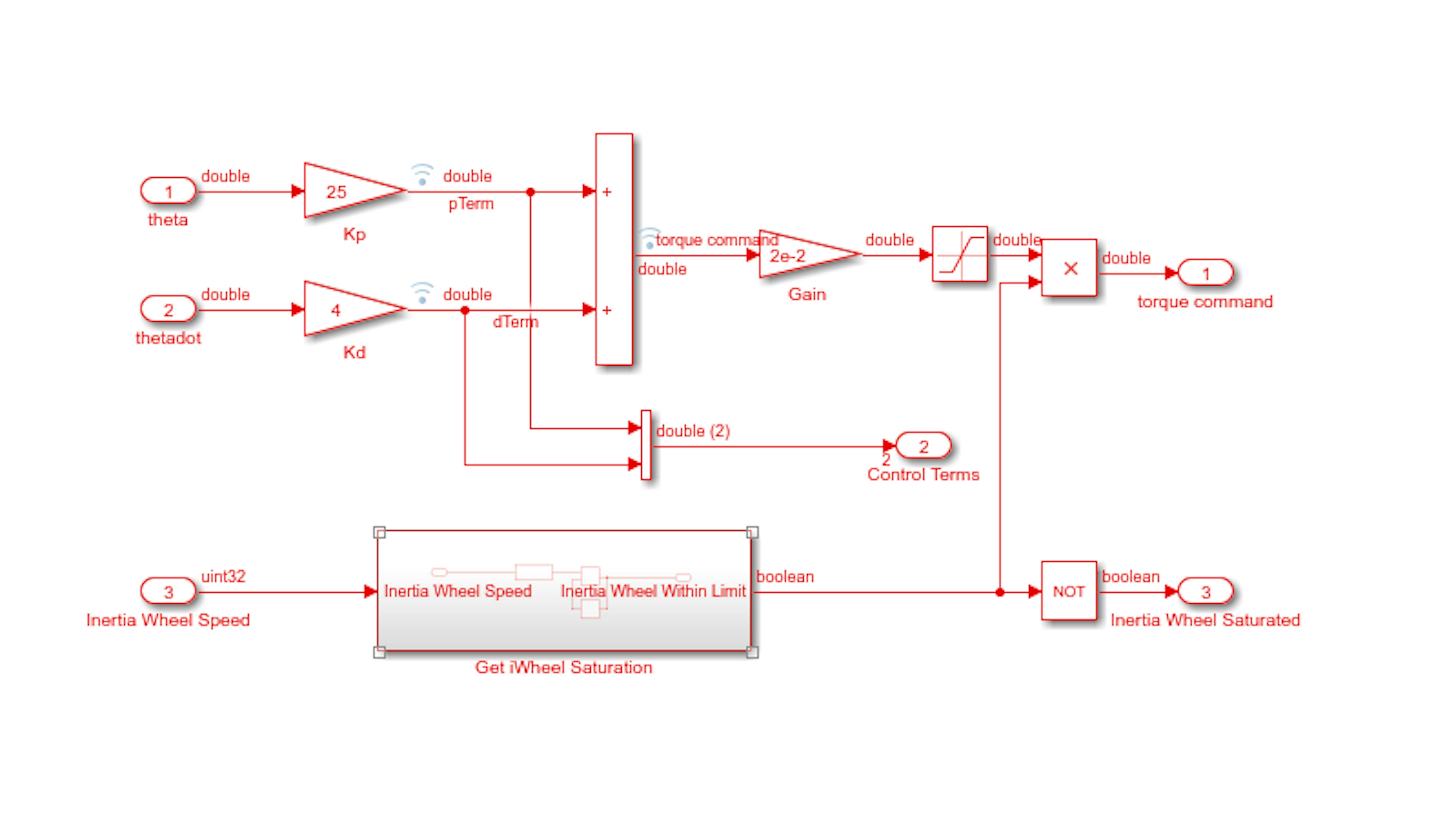
Now, let's think about what this is outputting. The value will be 1 when the inertia wheel is spinning, and 0 if it has saturated. The outport label is Inertia Wheel Saturated, which has the opposite implication. Therefore, you should negate this logical value before it reaches the Inertia Wheel Saturated output block. Add a Logical Operator block from Simulink → Logic and Bit Operations and set the logical operator to NOT. Connect the block as shown:
Go to the top level of the model, add a Display block from Simulink → Sinks, and connect it as shown. Resize the Display block because you will display a few more signals later. You may need to move some blocks and signals around to make room for the Display block:
Label the signal as shown above and run the model again. Enable the inertial wheel and lean the motorcycle all the way to the kickstand from the vertical position. You will see that the inertia wheel speed ramps up like before and also make sure to Observe the Display block switch from 0 to 1 when the threshold is met. Disable the inertia wheel using the manual switch and Stop the model.
Stop on extreme lean angles
Next, let’s program the controller to shut off the inertia wheel motor when θ is far from zero. Run the model if it is not already running.

Examine theta in the Scope window. Lean the motorcycle on its kickstand and note the range of θ:
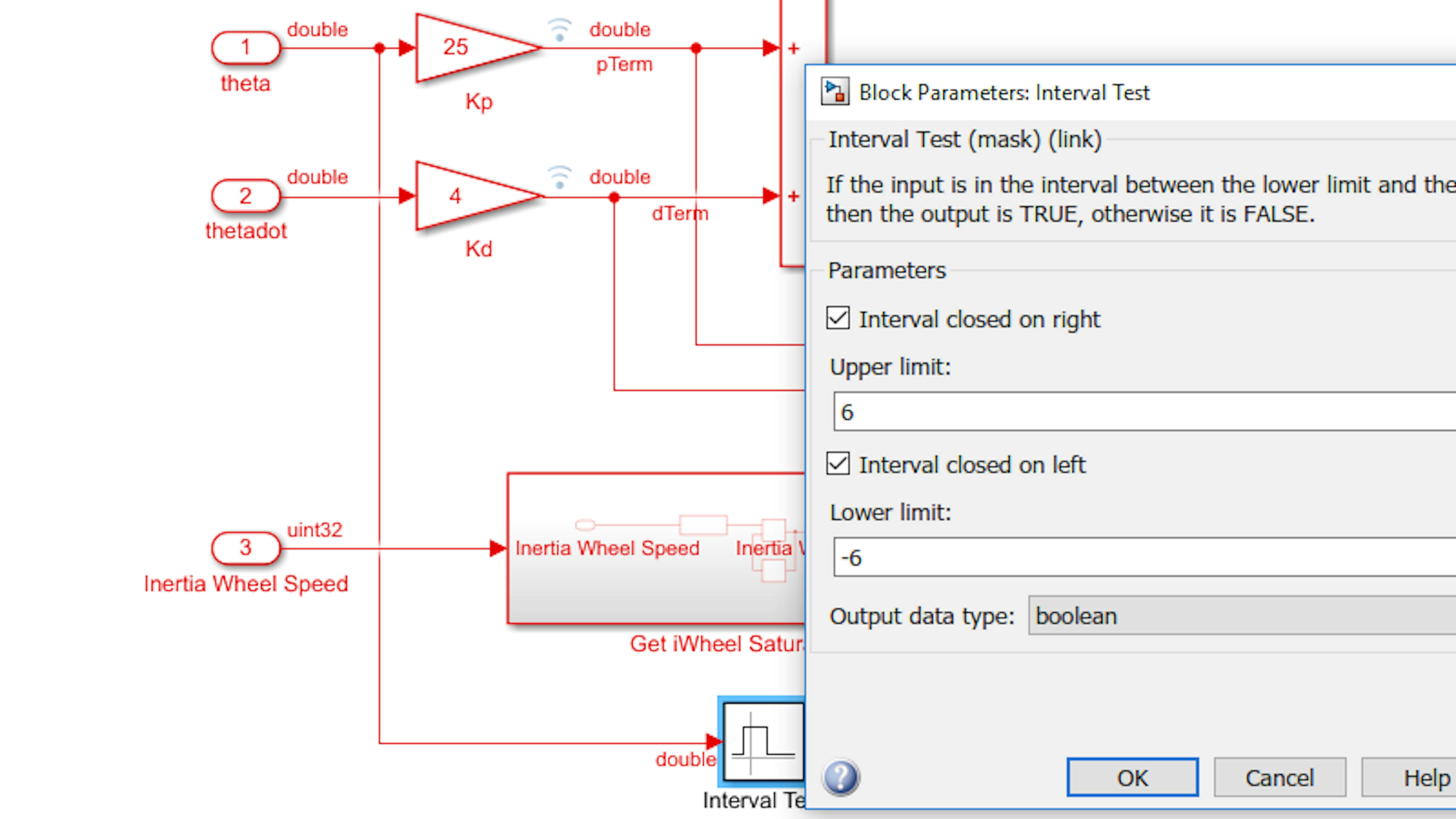
It is safe to say that if the lean angle reaches either of these extremes, the motorcycle is not in a stable balancing mode and cannot reverse direction with just the inertia wheel. We will consider the motorcycle to be “fallen” if the magnitude of the lean angle exceeds 6 degrees and therefore turn off the inertia wheel.
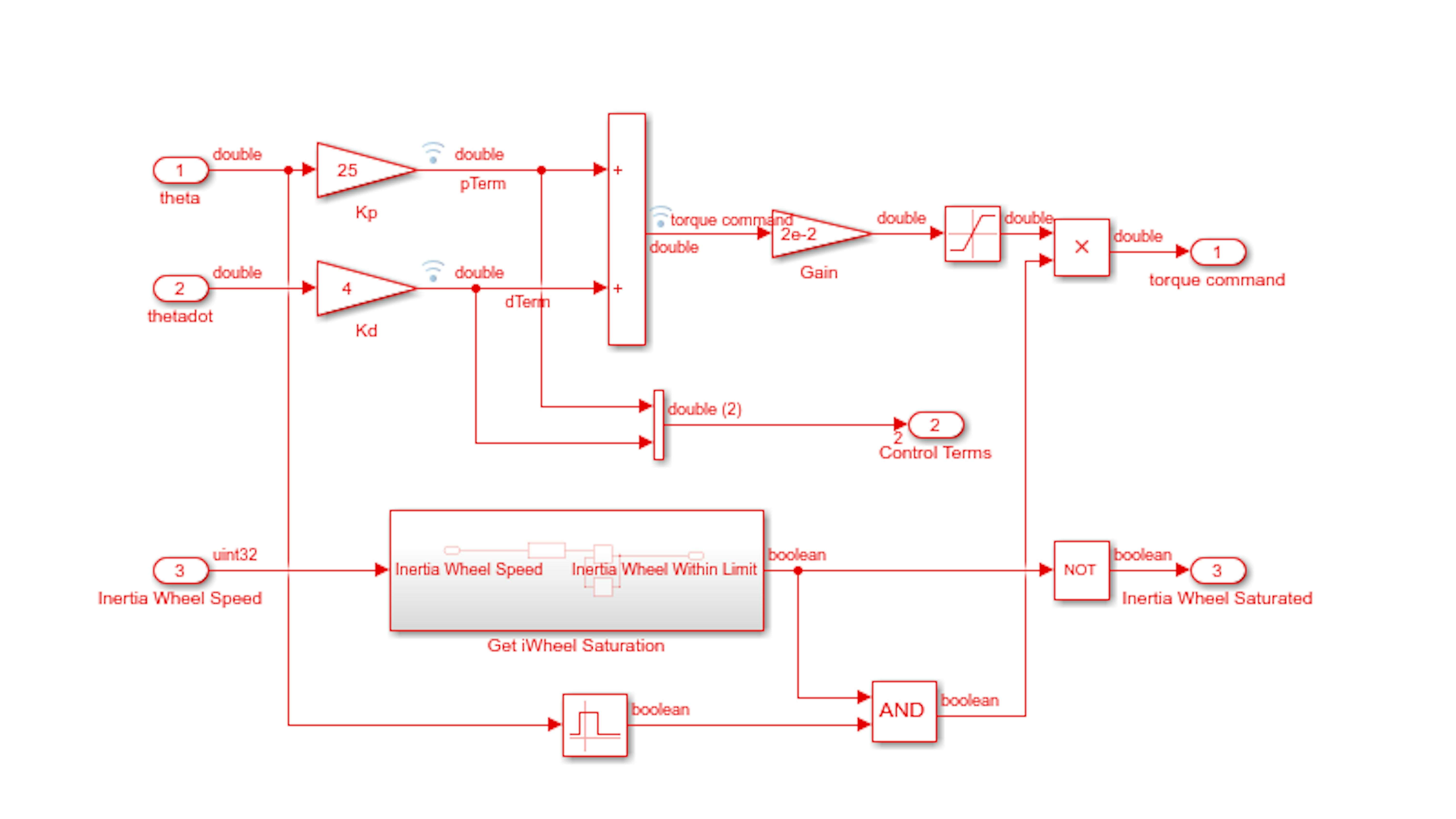
To do this, stop the model, and access the Controller subsystem. Add an Interval Test block from Simulink → Logic and Bit Operations and branch the theta signal to connect it. Set the interval test limits as shown and then Press Apply and OK:
The output of the Interval Test block is a logical value of 0 or 1. The inertia wheel motor should be enabled only if both the inertia wheel speed is below the threshold and the lean angle is within 10 degrees of θ = 0. To implement the AND logical gate, add a Logical Operator block from Simulink → Logic and Bit Operations. Route the signals as shown:
Let’s try it out. Run the model and enable the inertia wheel motor. Experiment with different lean angles and ensure that the inertia wheel motor does not drive when the motorcycle leans outside +/- 6 degrees from vertical.
Disable the inertia wheel motor and stop the model.
Let’s report the “fallen” status in the Display block like you did for the inertia wheel saturation status. The output of the Interval Test block is 1 when the lean angle is in an acceptable range and 0 when it is not. Since you are referring to the out-of-range status as “fallen,” you want the opposite of this signal. Copy and paste the Relational Operator block containing the NOT operator and add another Out1 block from Simulink → Sinks. Connect and label the blocks as shown:
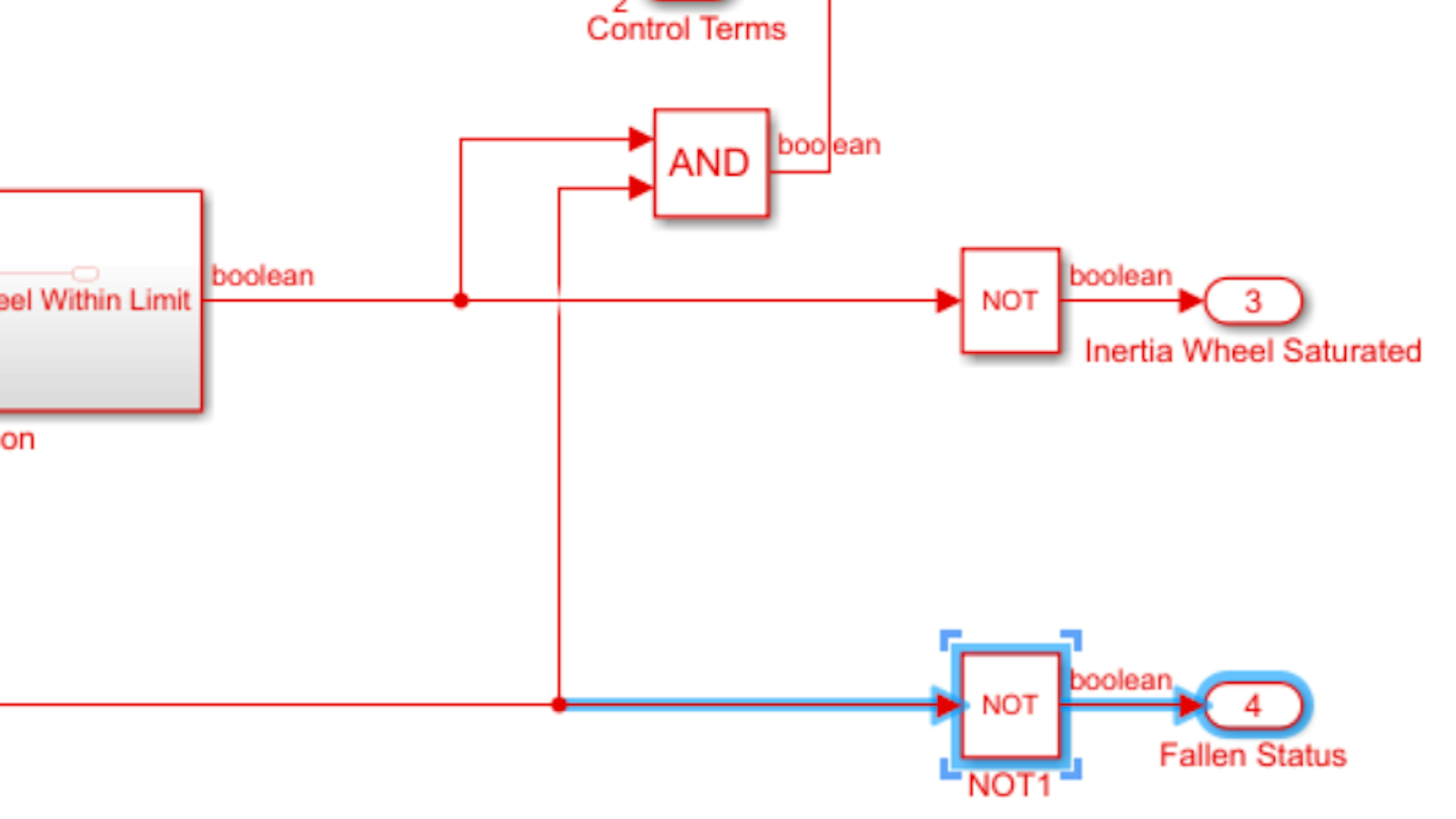
Now, return to the top level of the model. Add a Mux block from Simulink → Signal Routing, and connect and label the signals as shown:
Run the model and observe the “fallen” status in the Display block for different conditions - a) within and b) outside +/-6 degrees.
Stop unless IMU is calibrated
For the next failsafe measure, you want to make sure that the inertia wheel motor does not drive unless the IMU has been calibrated. In the previous exercise, you built some logic in the IMU subsystem to convert the four IMU status elements into a single true or false signal. The controller can use this information to enable or disable the inertia wheel.
To begin, let’s observe the behavior of the calibration status elements as well as the IMU Calibrated signal. Run the model if it is not already running and disable the inertia wheel motor. Observe the Calibration Status and Calibration Vector displays. Rotate the motorcycle about its principle axes until the Calibration Status display shows 1:
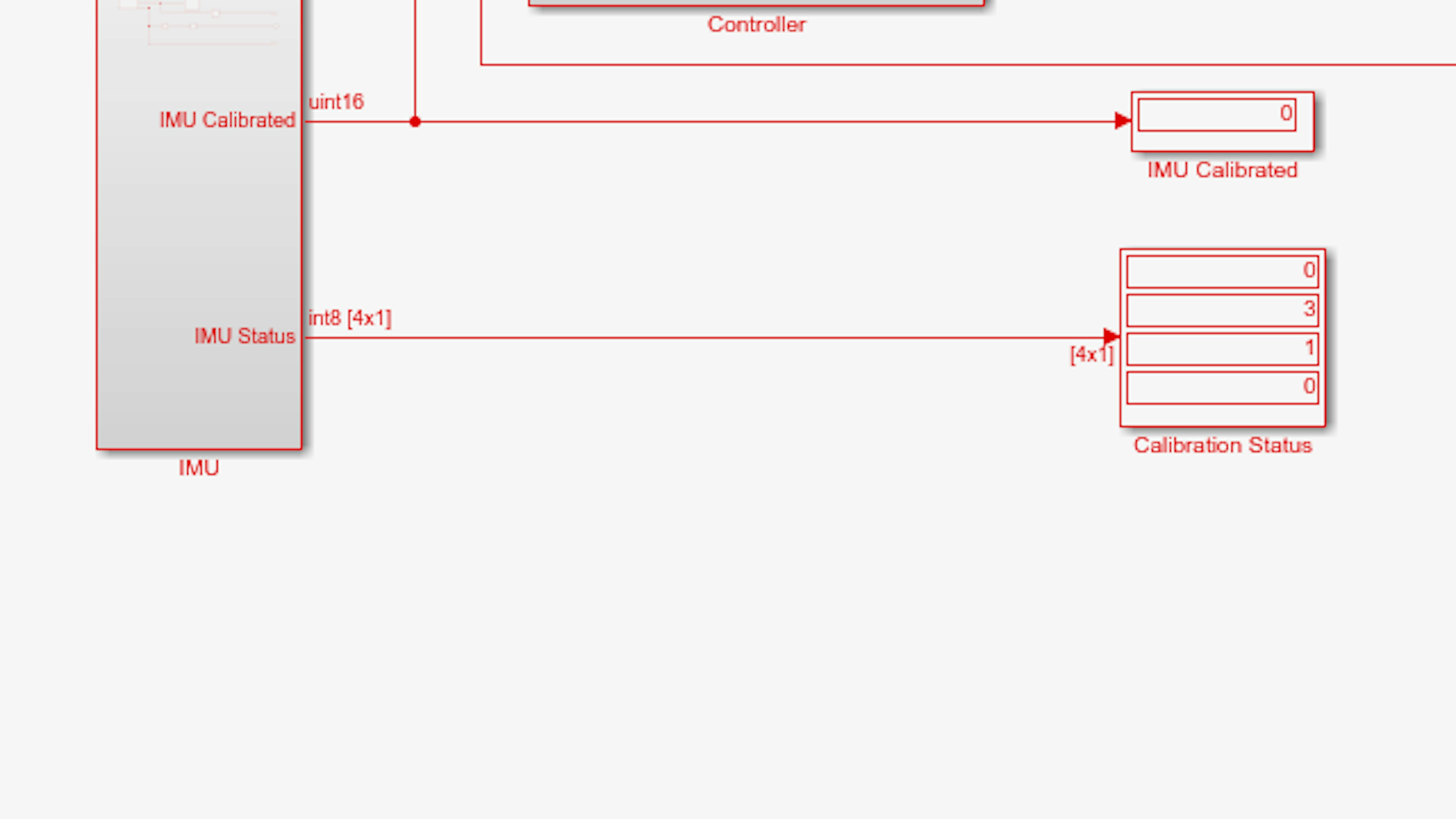

The IMU sometimes loses calibration to some degree for one or more sensors after it has initially been calibrated. For practical reasons, you want to consider the IMU to be calibrated if it has met the calibration thresholds at some time in the past within the current power session. Therefore, you want to latch the IMU Calibrated signal to a value of 1 as soon as the calibration thresholds are met for the first time and leave the signal at that value indefinitely.
Let’s proceed by providing an inport for the IMU Calibrated signal. Stop the model. Branch the IMU Calibrated signal and label it as shown:
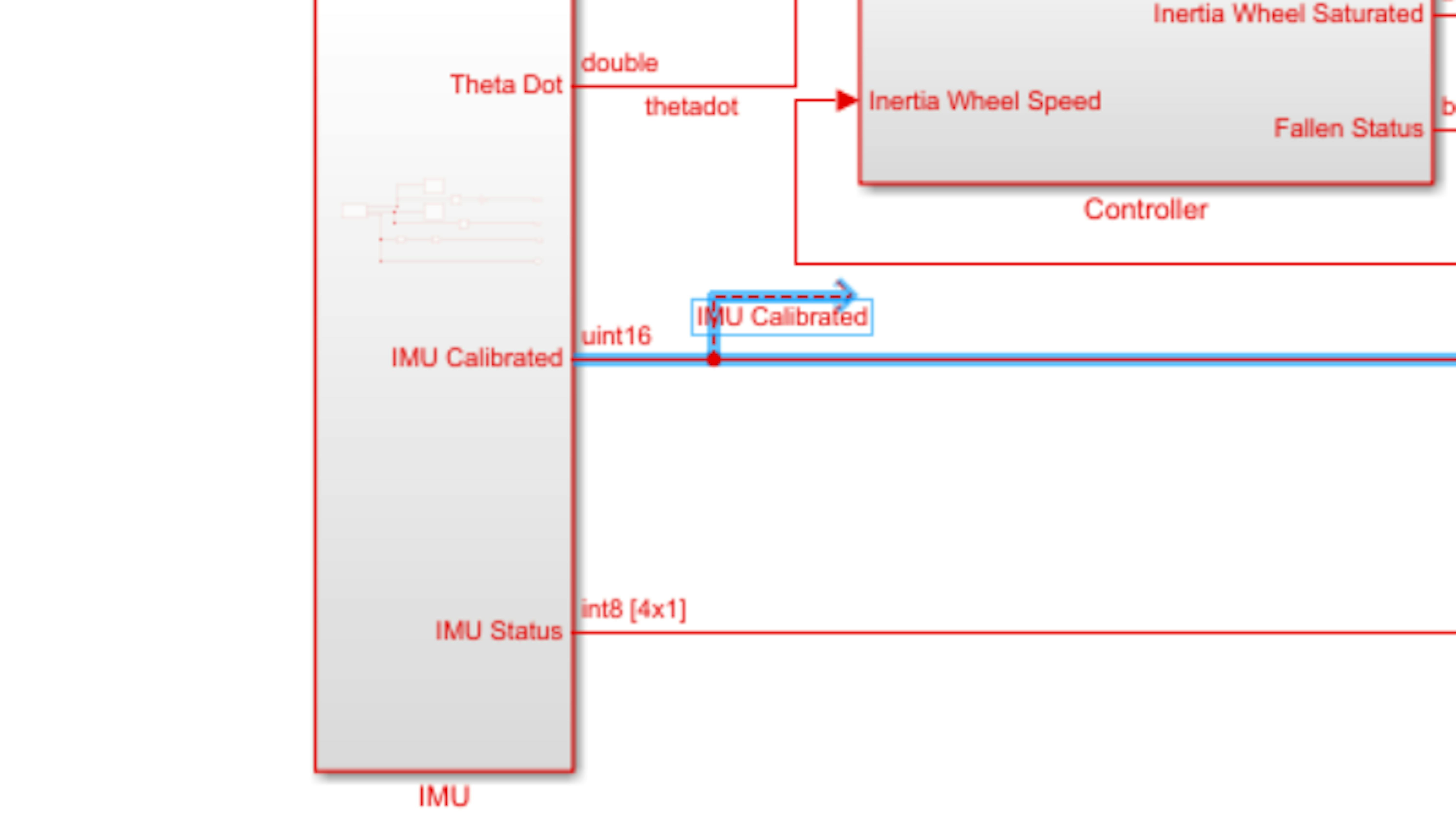
Now, drag the signal into the Controller subsystem, creating a new inport in the fourth position:
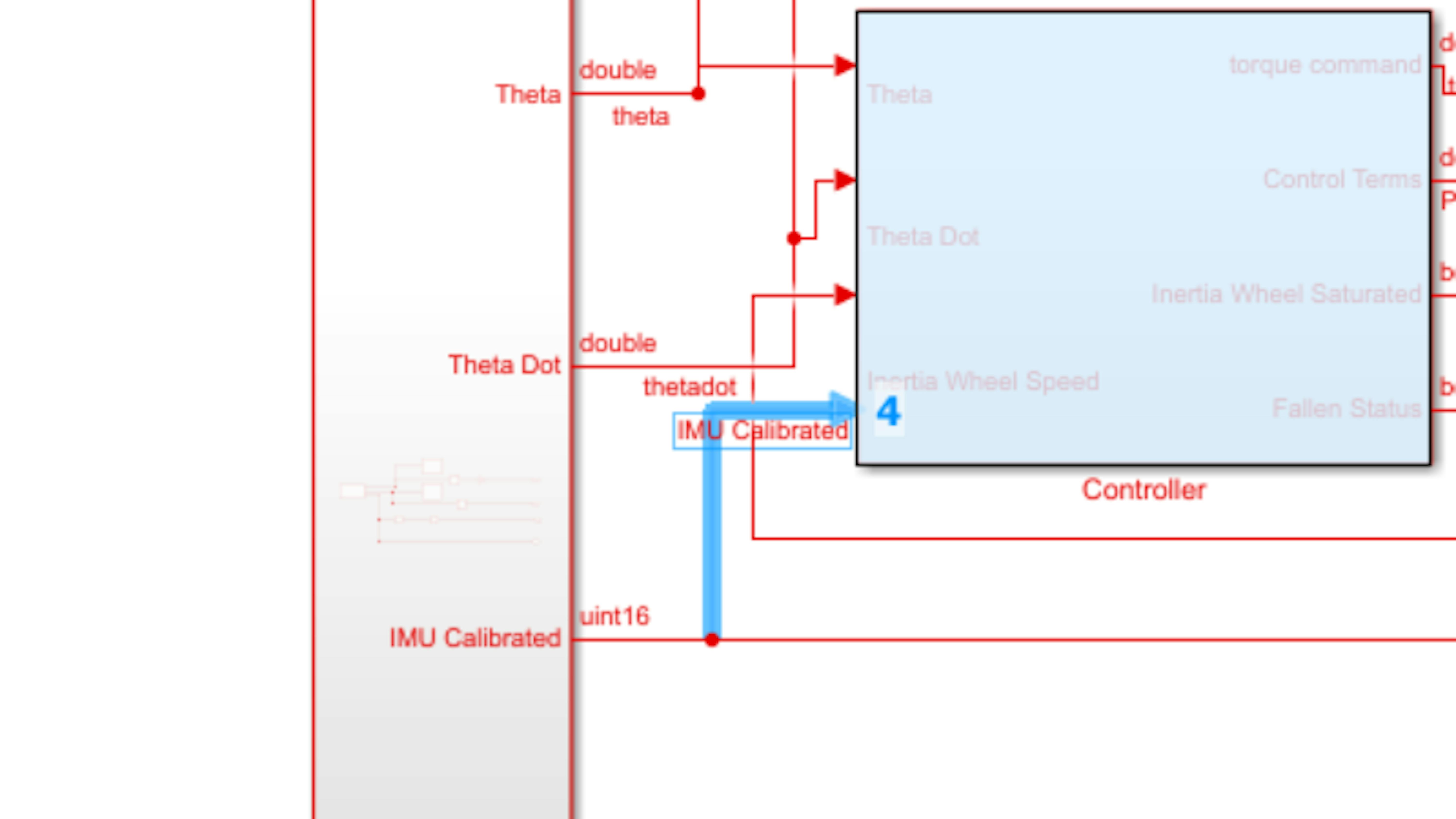
To latch the IMU Calibrated signal, go into the Controller subsystem and add a Unit Delay block from Simulink → Discrete and a Logical Operator block from Simulink → Logic and Bit Operations. Set Operator to OR.
Select the* Unit Delay* block and press Ctrl + I to reverse its orientation. Then, route and label the signals as shown:
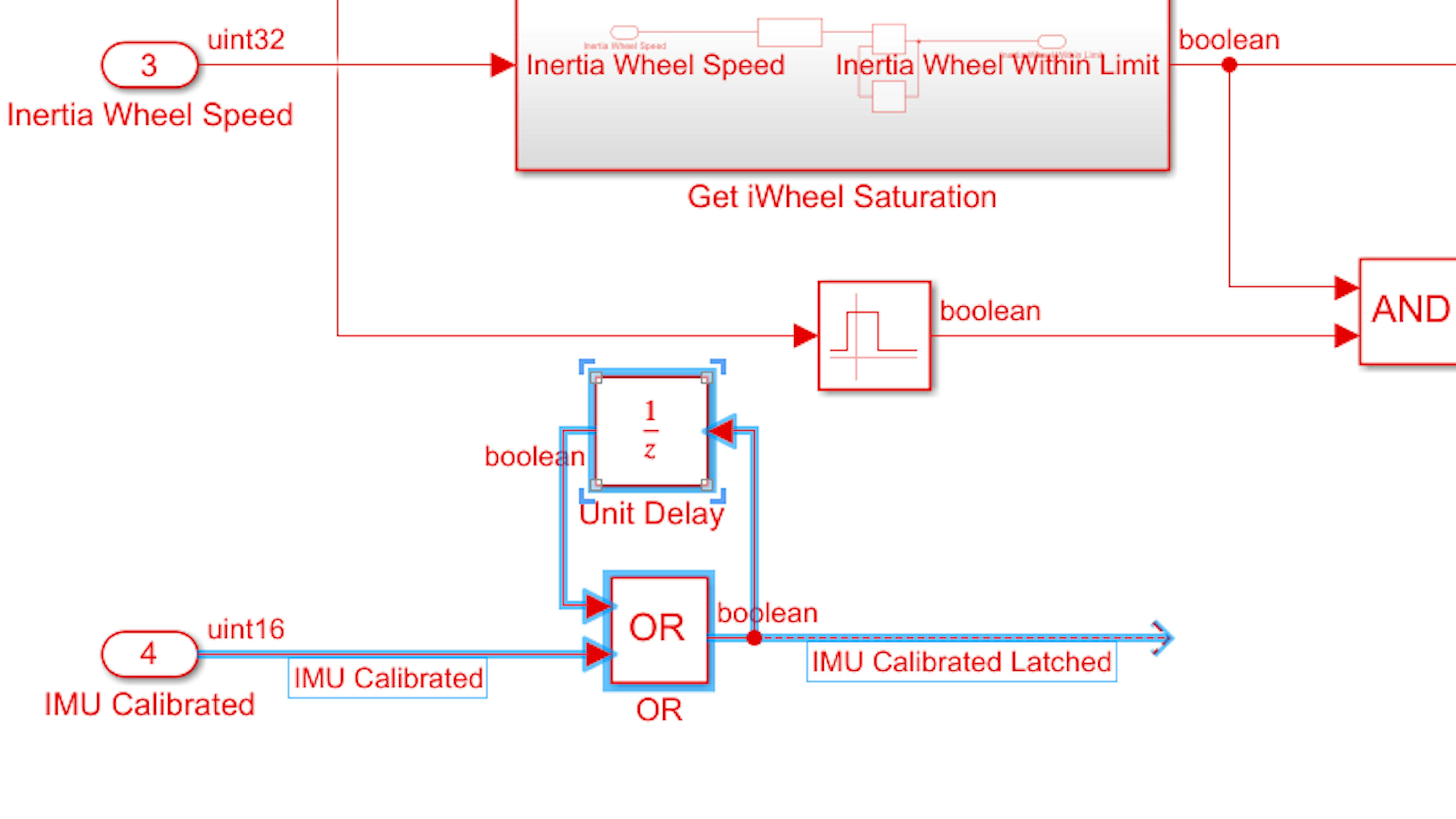
Spend some time thinking about how this mechanism will permanently latch the output signal to 1 as soon as the IMU calibration thresholds are met for the first time.
Now drag the IMU Calibrated Latched signal to position 3 on the AND Logical Operator block, creating a new inport:
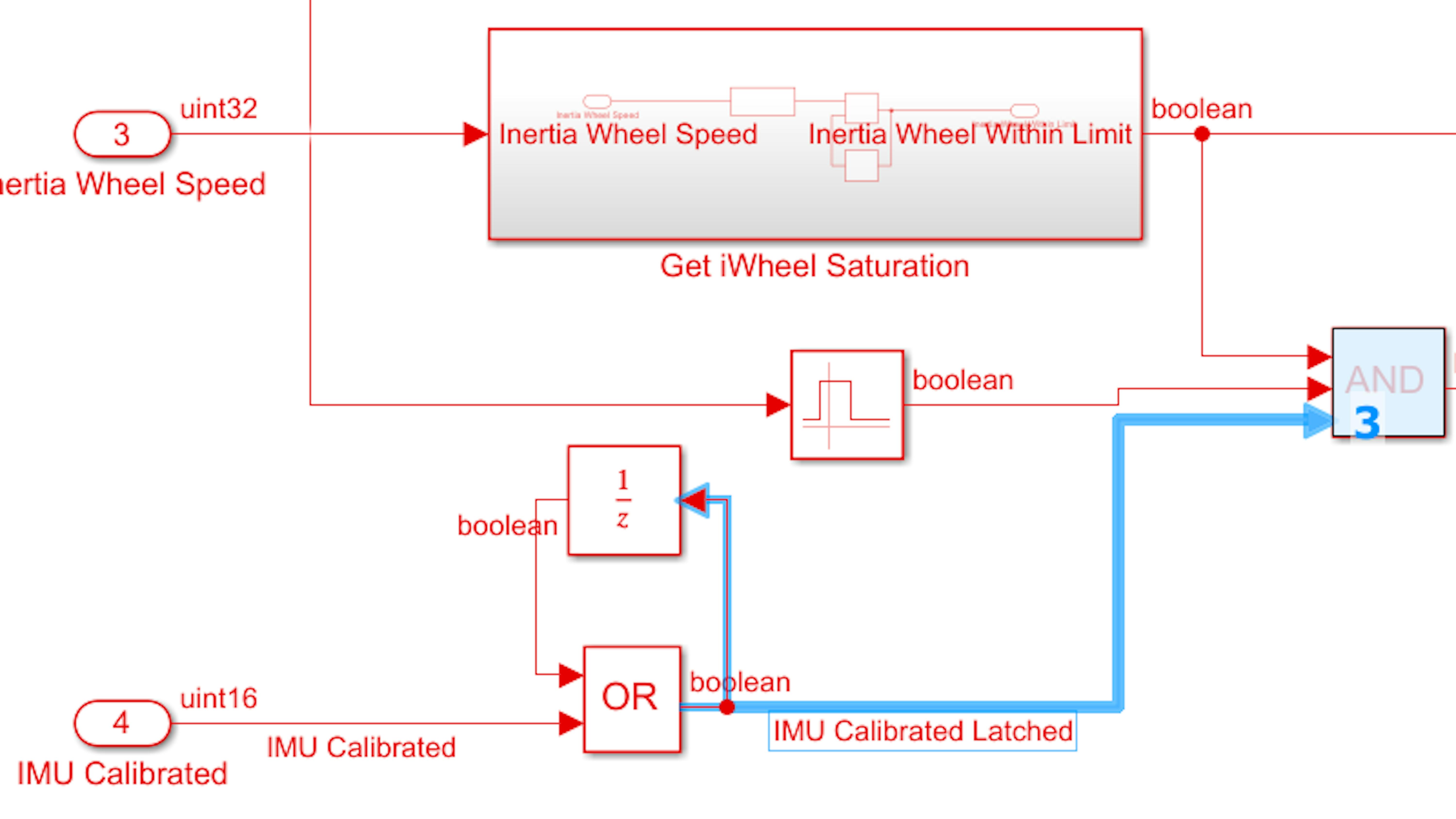
Finally, let’s add this status to the Display, along with the first two failsafe modes. In the Controller subsystem, add an Out1 block from Simulink → Sinks, and label and connect it as shown:
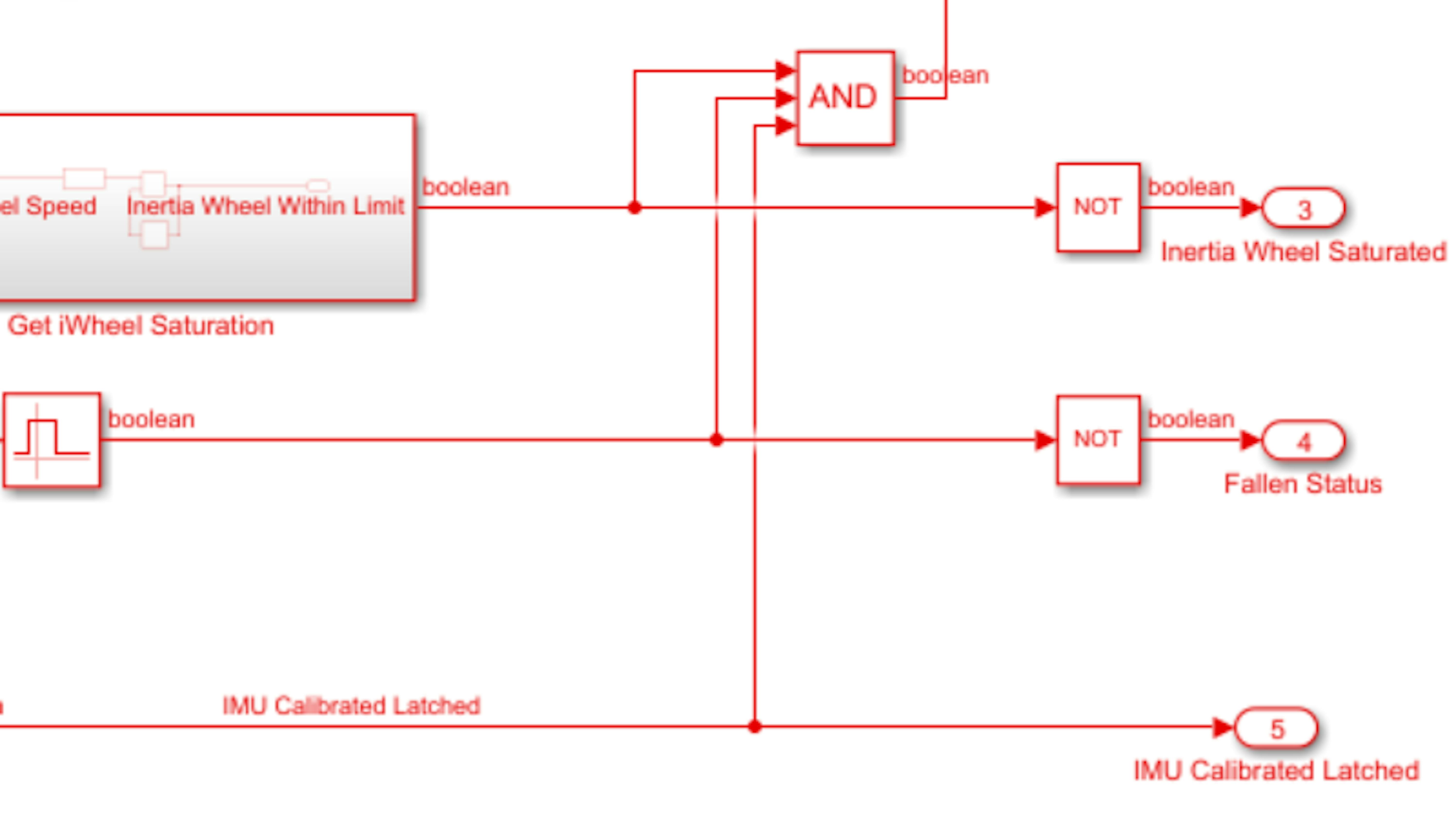
Return to the top level of the model and connect the IMU Calibrated Latched outport to the Mux block, creating a third inport:
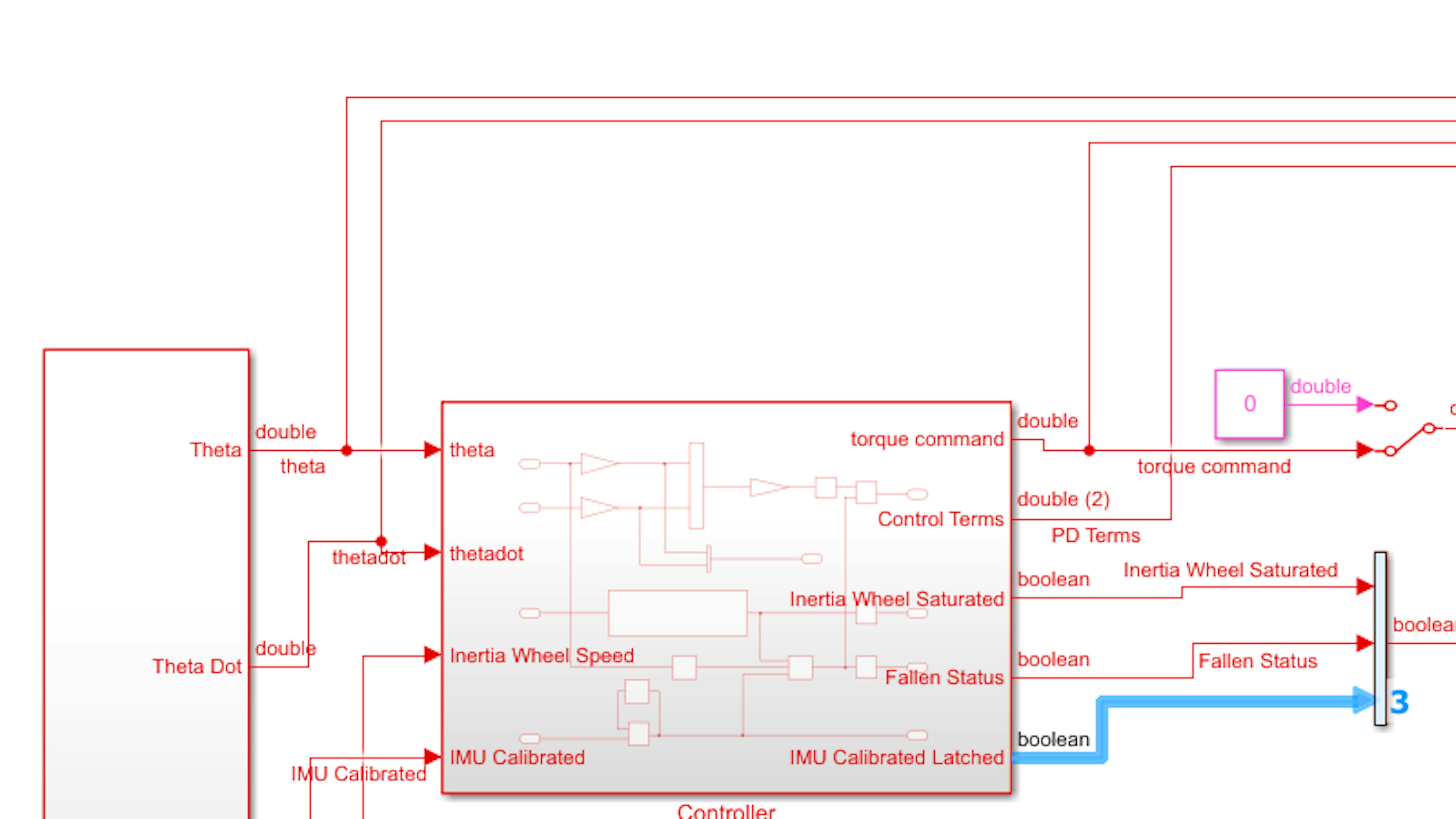
Label the new signal IMU Calibrated Latched:

Next, disrupt the power to the IMU by turning off the motor carrier and unplugging the USB cable from your computer. Restore the motor carrier power and USB cable.
Run the model and enable the inertia wheel motor using the manual switch. Ensure that the inertia wheel motor does not begin to drive until the IMU Calibrated signal hits 1 for the first time. Check the failure status displays to ensure that the IMU Calibrated Latched signal remains at 1 permanently once it latches. Make sure the other two failsafe mechanisms (inertia wheel speed cutoff and “fall” sensing) still work as before.
When you are finished, disable the inertia wheel motor and stop the model.
Shut down if low power
Now, let’s add the final failsafe feature: shutting off the inertia wheel when the battery level is too low. Operating the inertia wheel with insufficient battery charge can damage the motor hardware since it will not be able to supply enough torque to correct the lean angle in the way it was designed. While the controller will automatically account for environmental variations, including slightly decreased motor torque, a significantly low battery level is outside the range at which the controller is stable.
When you are working on your Simulink models between runs on the MKR1000 (especially runs where you are using motors), it is a great time to remove the battery from the motor carrier and charge it. It is important to never let these batteries lose too much charge, or they can become permanently damaged or even unrechargeable

Let’s begin by monitoring the battery level. In the Simulink Library Browser, navigate to the Simulink Support for Arduino MKR Motor Carrier library and drag the Battery Read block into myNewMoto.slx. Configure the block as shown:
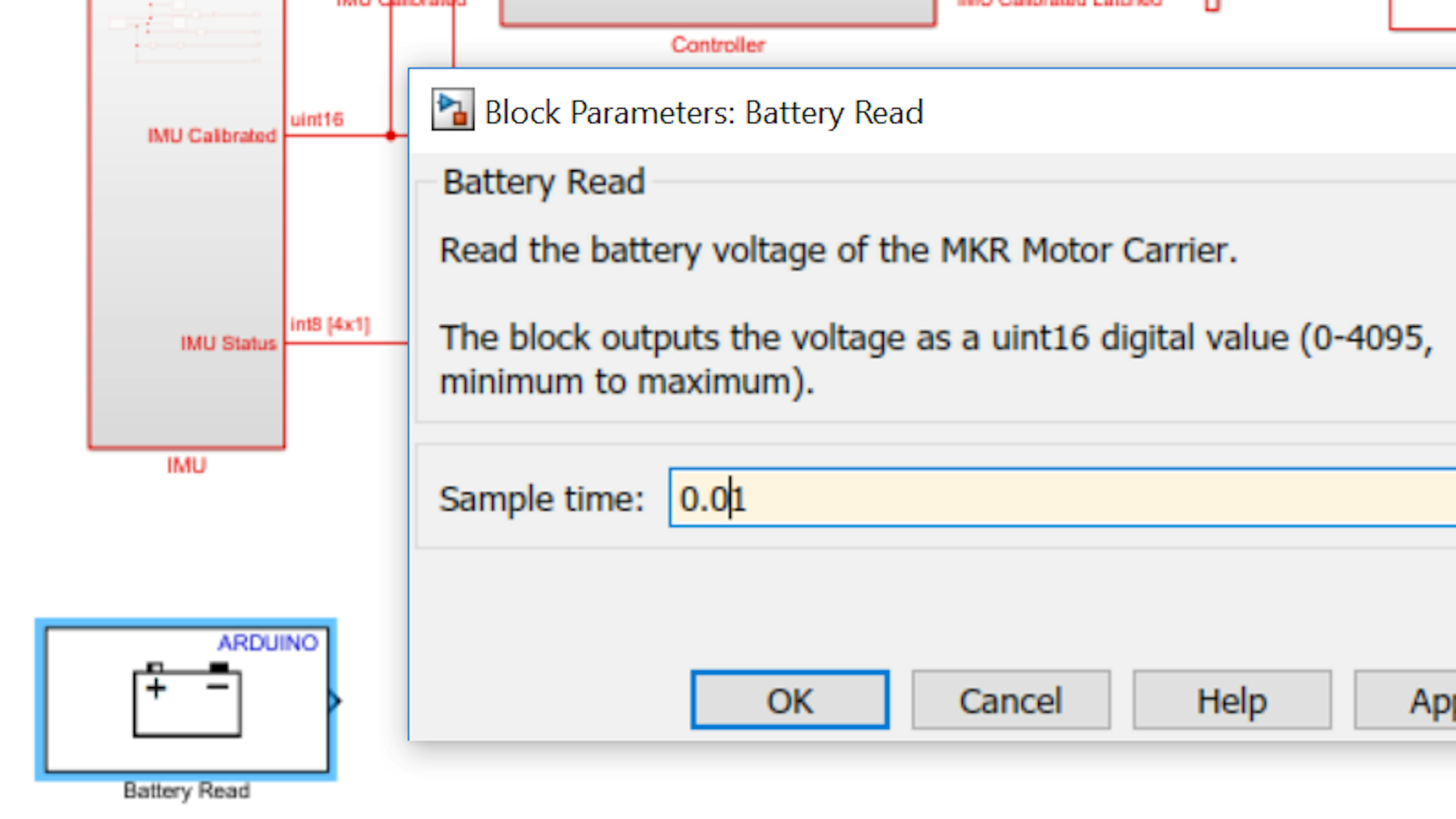
The output is an integer read directly from a battery charge sensor on the motor carrier. This integer is equal to the 77 times the physical voltage of the battery in volts.
Add a Display block from Simulink → Sinks, and connect it to the Battery Read block. Label the Display block as shown. Then, disable the inertia wheel motor, and run the model:
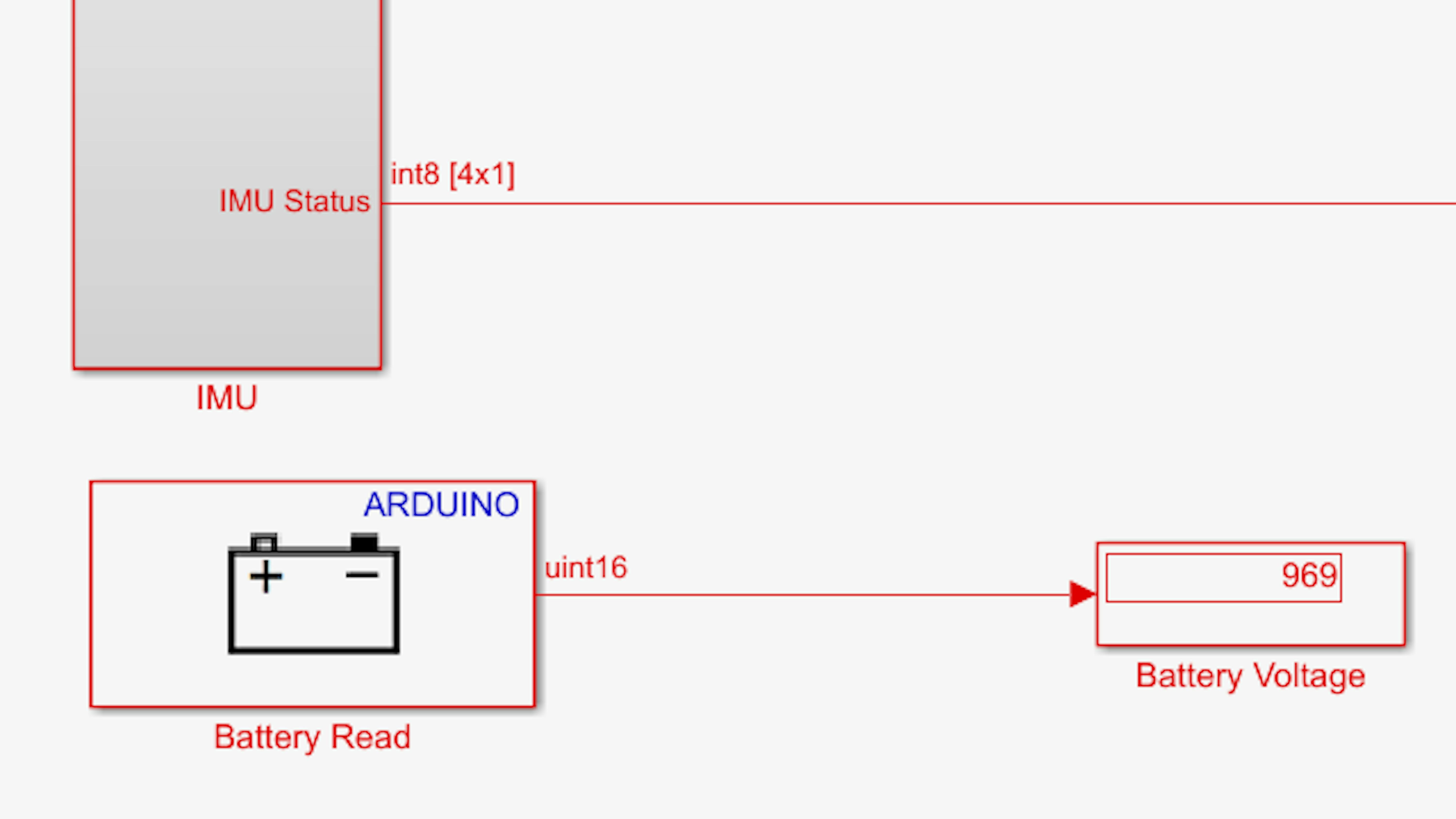
Note: You might observe a small amount of noise in the voltage measurement even when the motor is not being driven, which is expected in any electrical measurement.
Notice that the data type of the battery measurement is a 32-bit unsigned integer (uint32). To convert the value to a real-world voltage, you will need a floating-point data type that can represent non-integers. Stop the model and add a Data Type Conversion block from Simulink → Signal Attributes and a Gain block from Simulink → Math Operations. Set the gain value to 1/77. Connect the blocks and label the final signal as ‘Battery Read’ as shown below. Run the model:
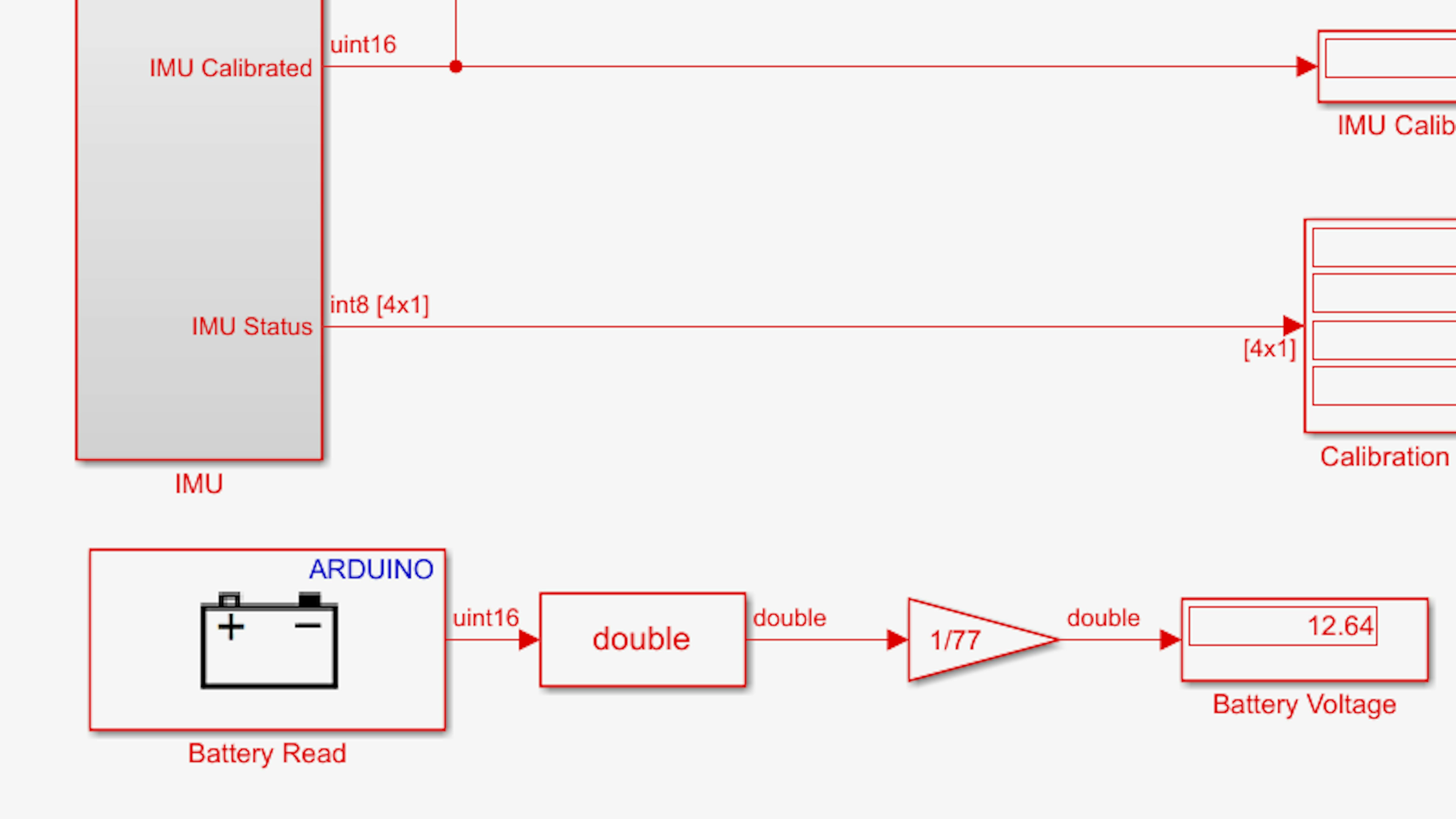
If the battery is fully charged, you should have a reading of at least 12 V. This is optimal for the inertia wheel motor to work properly, but a voltage as low as 11 V is acceptable. Now, see what happens to the voltage while the motor is being driven. With the model still running and the inertia wheel still disabled, calibrate the IMU by turning it at least 90 degrees along each axis until you see the Display block to the right of the Controller subsystem show 1 for the IMU Calibrated Latched signal:
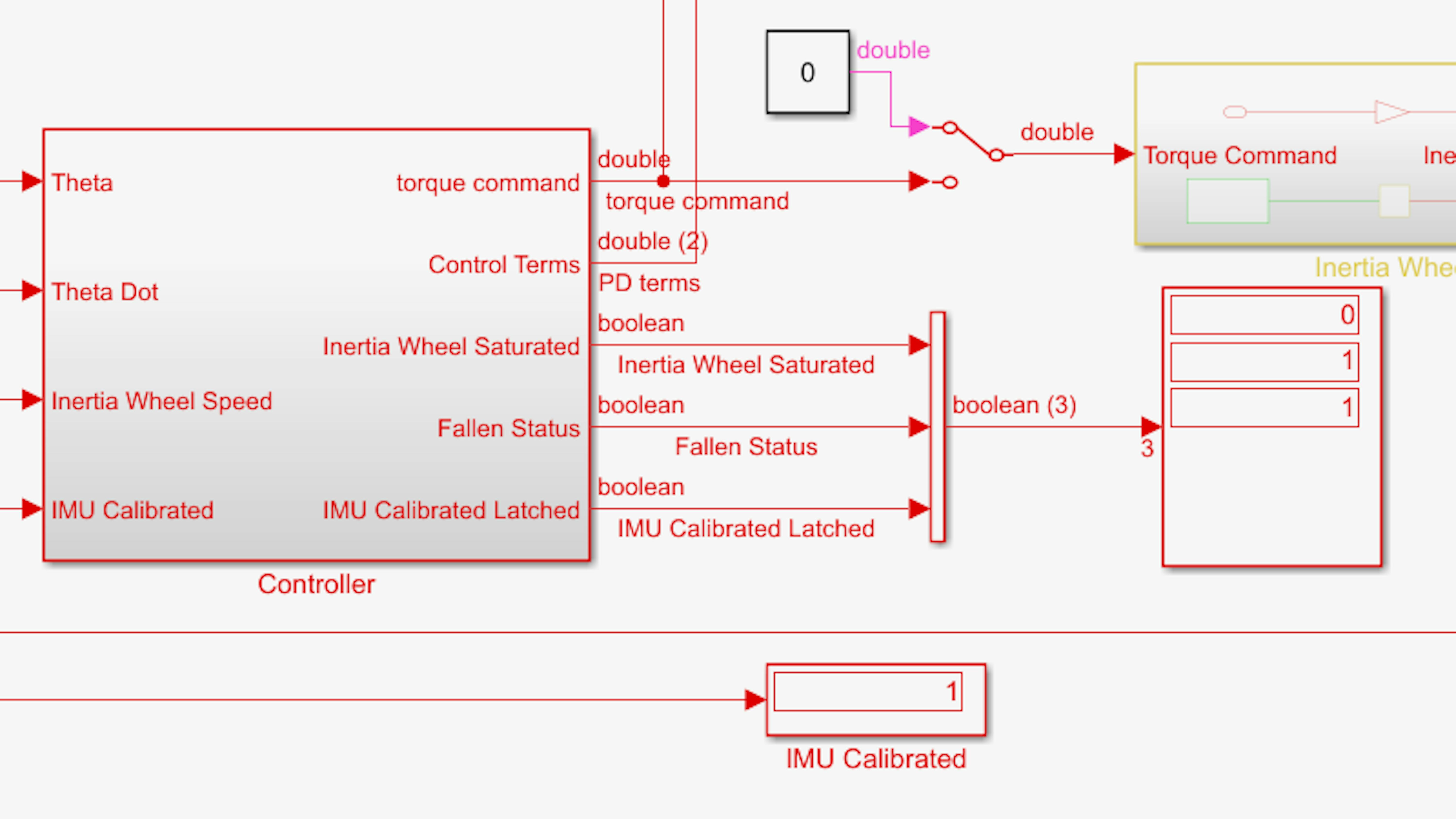
Now, enable the inertia wheel motor and hold the motorcycle near θ = 0 while watching the Battery Voltage display. Try leaning the motorcycle a few degrees in either direction so that the motor drives some torque to the inertia wheel:

Disable the inertia wheel motor and stop the model.
What happens to the battery voltage while the motor is driving? A battery at rest (or close to it) has a higher voltage than a battery that is actively driving a motor due to back electromotive force (back EMF), which is a consequence of Lenz’s Law.
Due to this phenomenon, you should consider an expected drop in voltage, as well as occasional dips and spikes in the voltage, when setting the threshold for the battery charge failsafe feature. For the purposes of this project, the lowest safe voltage for any portion of the application’s life span will be 10.5 V.
To implement this logic, branch the converted battery voltage (after the Gain block) to the Controller subsystem, creating a fifth inport:
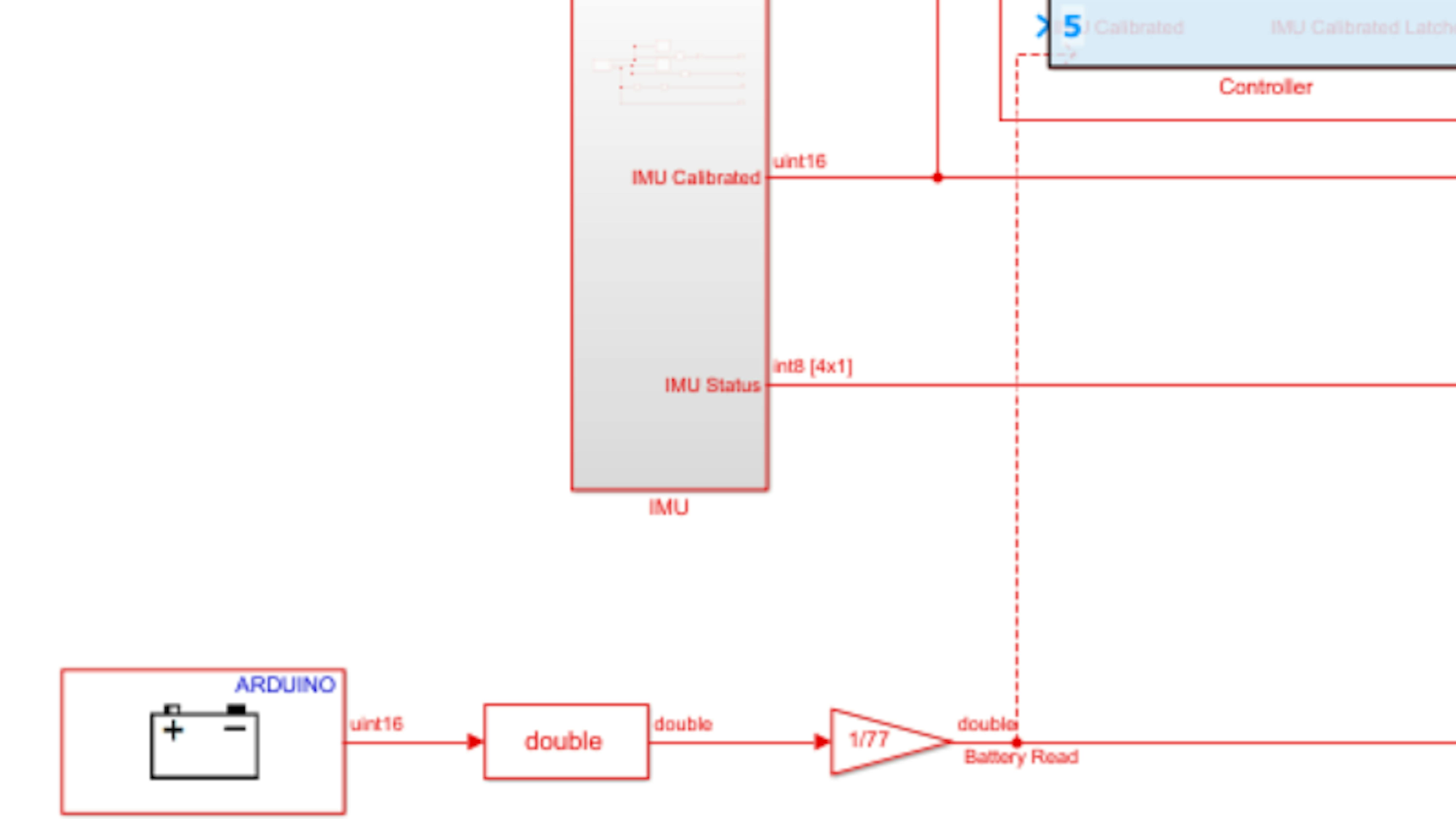
Next, access the Controller subsystem, find the new Battery Read inport block, and move it to the lower left corner. To compare the battery voltage to the threshold described earlier, add a Compare To Constant block from Simulink → Logic and Bit Operations, and configure and connect it as shown
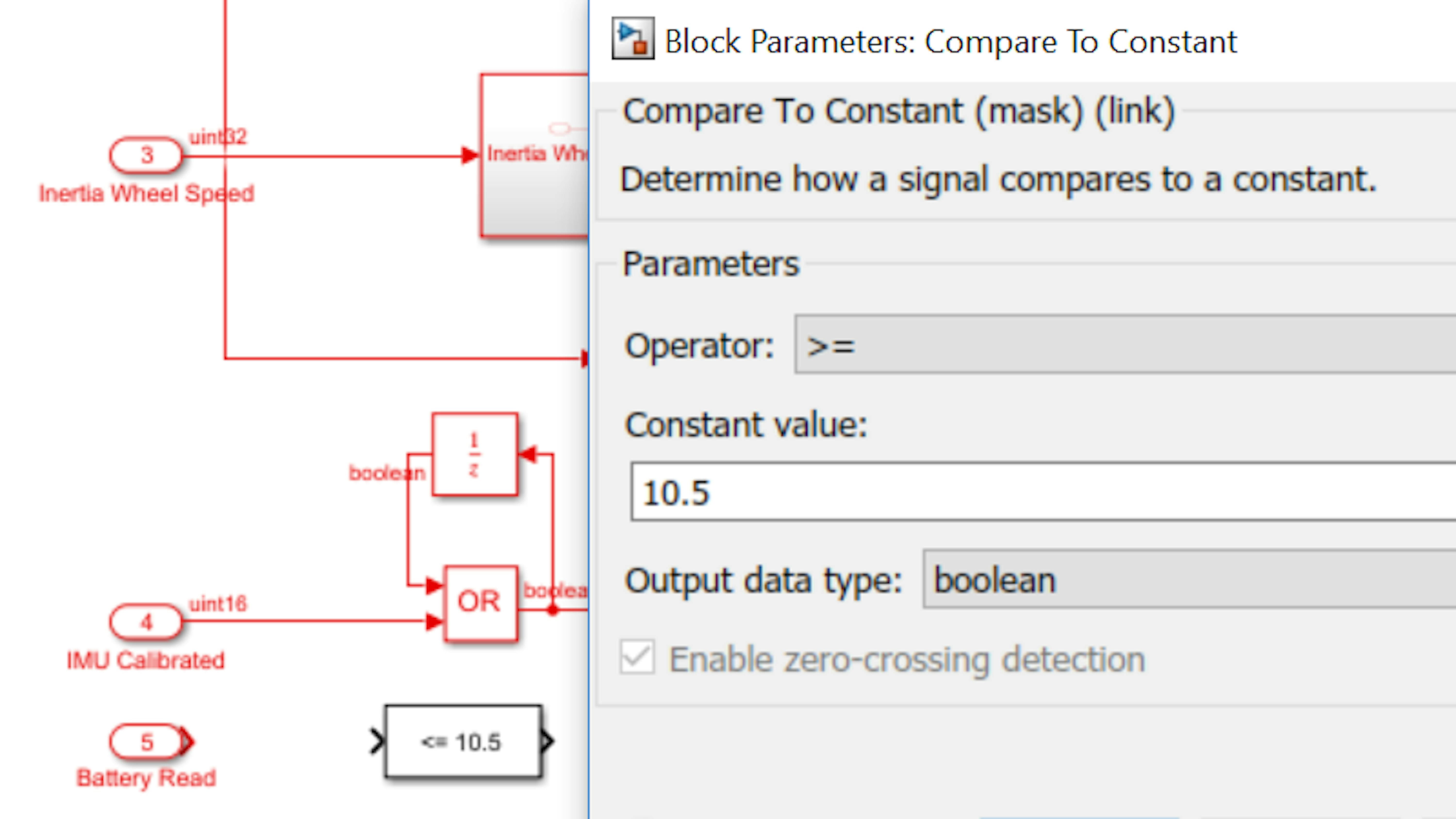
The output of the Compare To Constant block indicates whether the battery is sufficiently charged at each moment in time. However, you want the “Battery Charged” signal to go to zero permanently after the first instance of a low battery detection even if the charge goes back above the voltage threshold. Due to the noise in the voltage measurement, the voltage will oscillate around the threshold randomly as it starts to generally drop. This can cause the inertia wheel motor to “sputter” as it turns on and off rapidly, which is not good for balance, or for the motor.
Therefore, you will want to latch off this signal so that the first instance of low voltage brings the “Battery Charged” signal permanently to 0. When this occurs, you should remove the battery from the motor carrier and charge it until full.
To latch the signal to zero when the battery first becomes undercharged, add a Logical Operator block from Simulink → Logic and Bit Operations, set the operator to AND, and add a Unit Delay block from Simulink → Discrete. In the Unit Delay block, set Initial Condition to 1. Connect the blocks as shown:
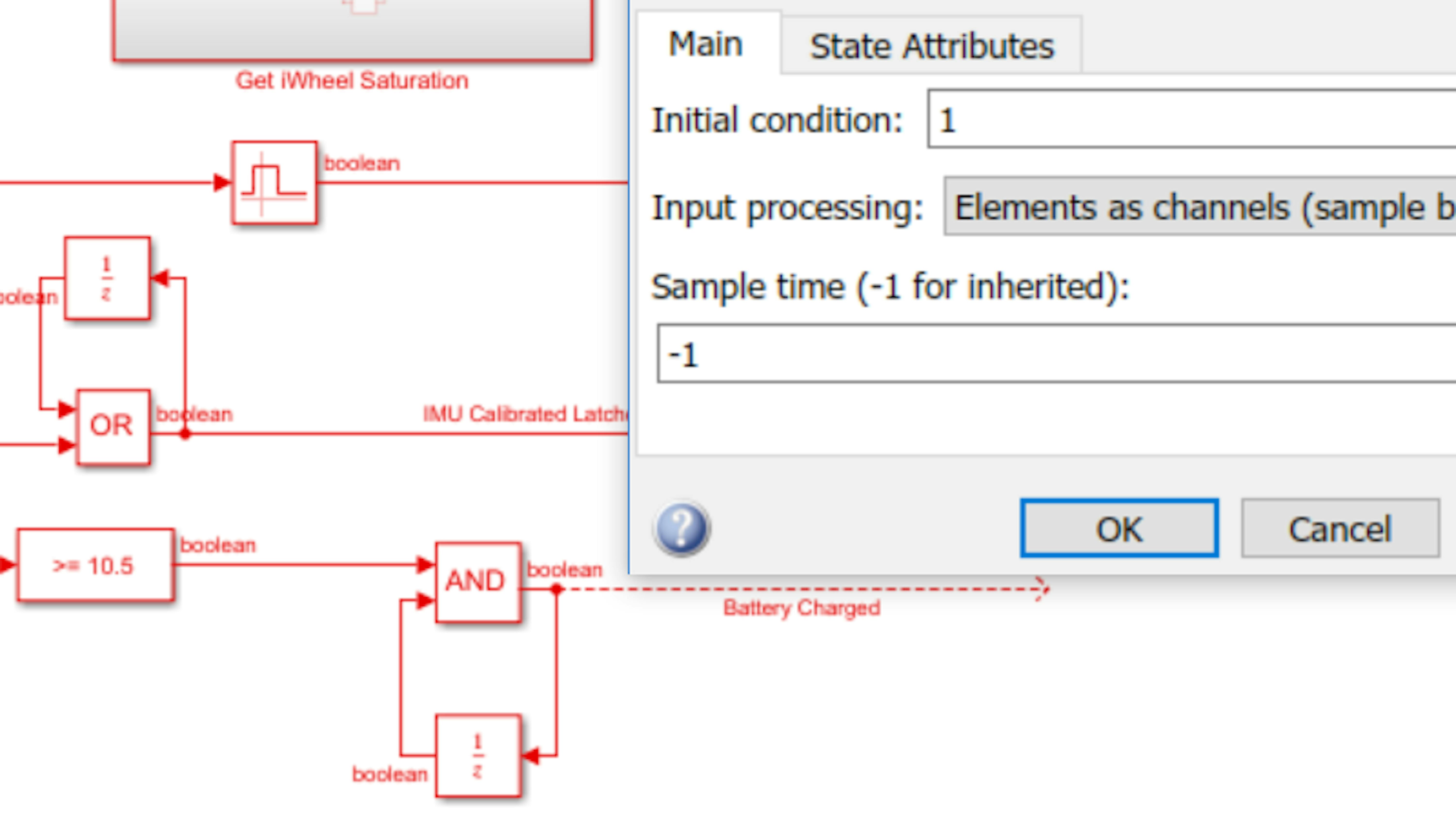
Route the Battery Charged signal into the central Logical Operator (AND) block, creating a fourth inport:
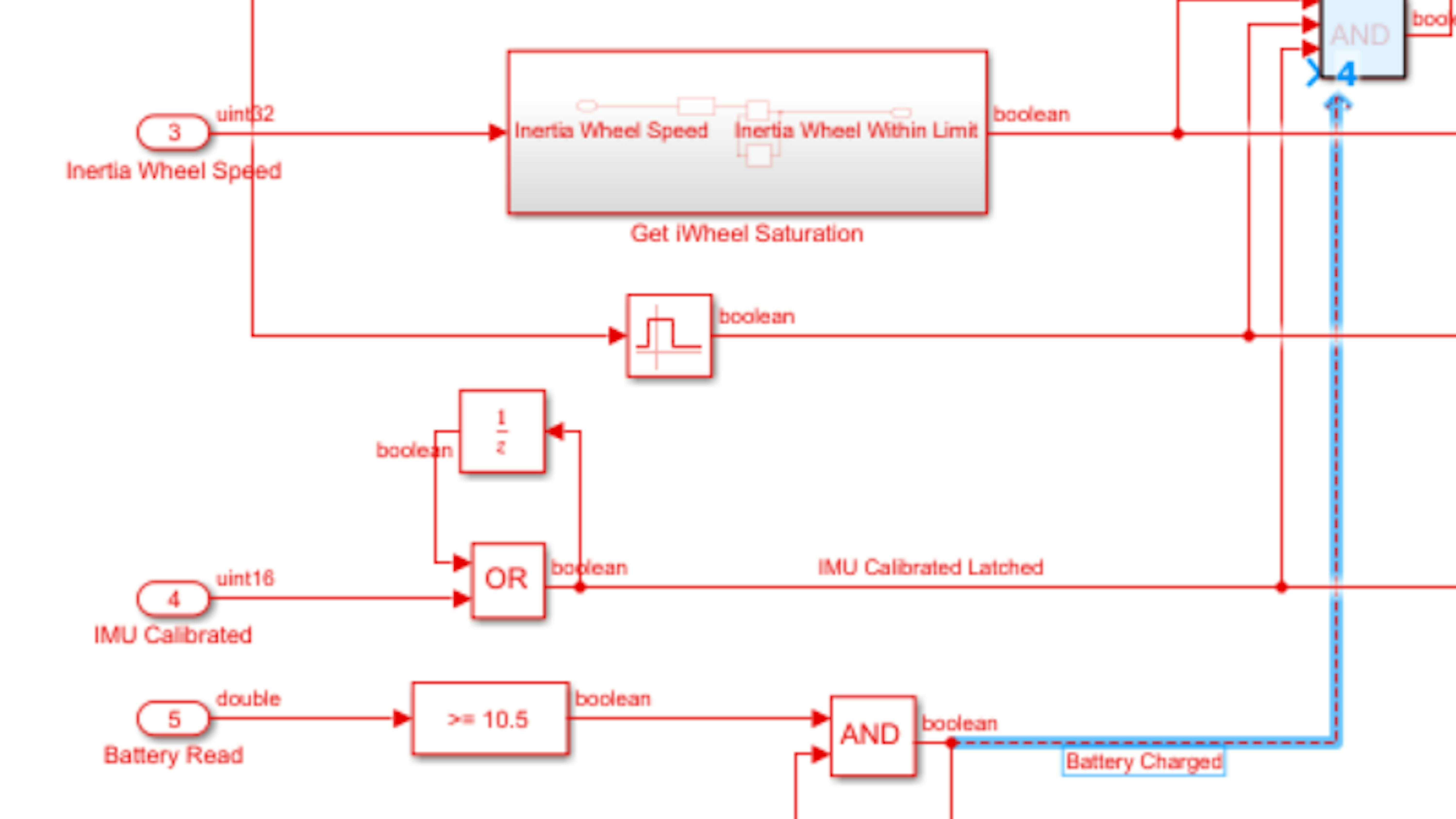
Add an Out1 block from Simulink → Sinks and connect and label as shown:
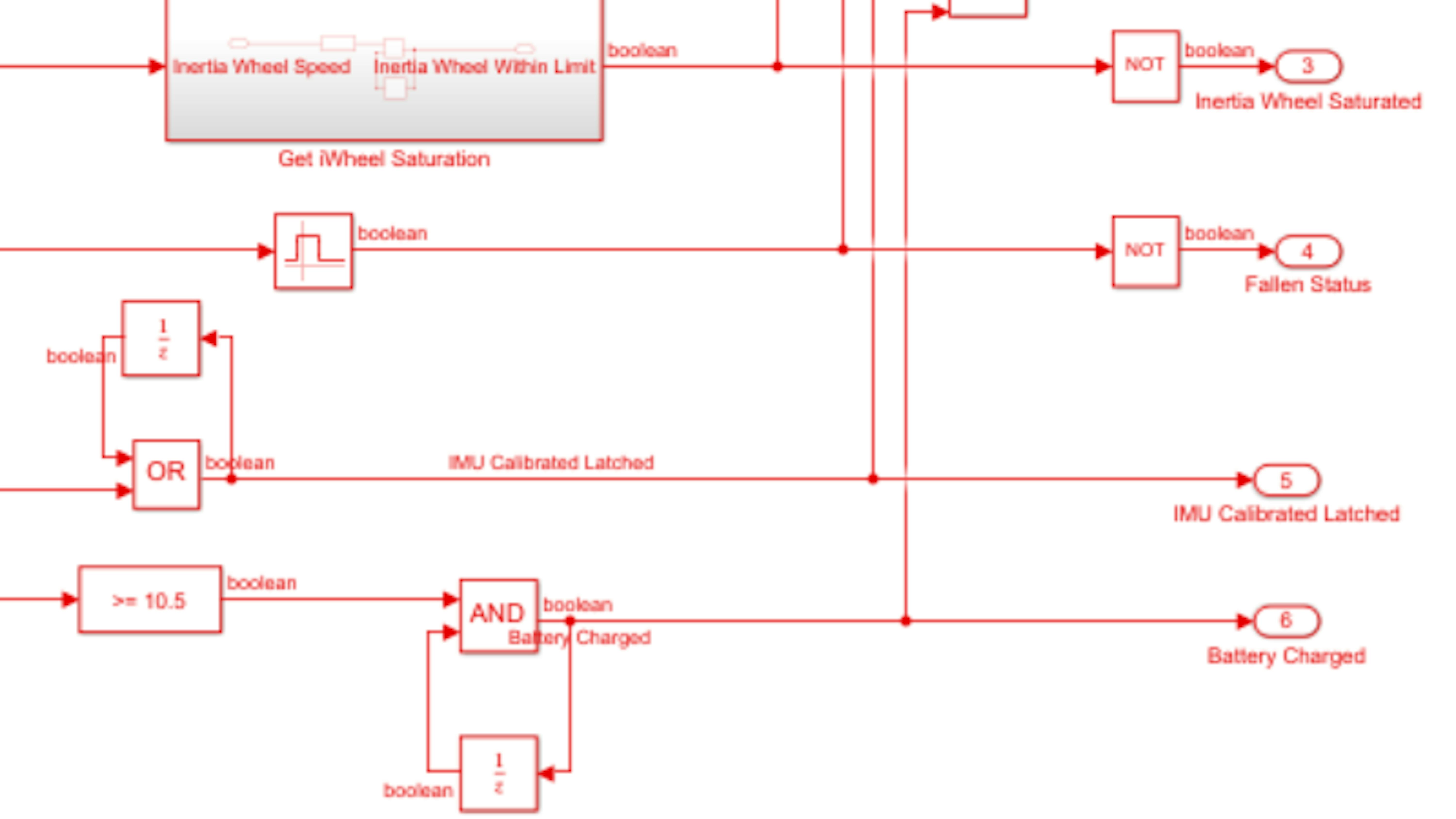
Finally, return to the top level of the model and drag the Battery Charged signal to the Mux block, creating a fourth input:
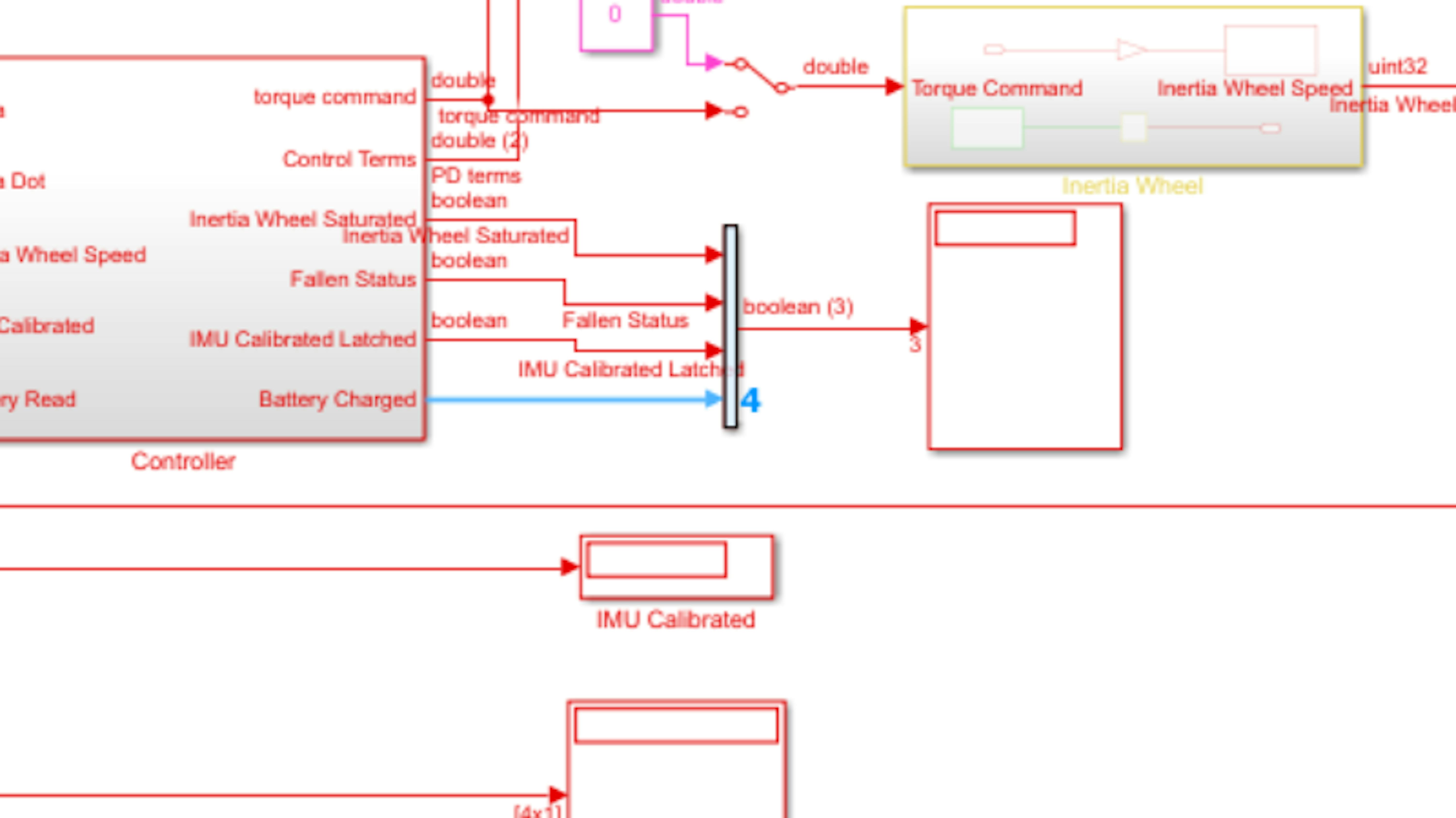
Label the signal Battery Charged, attach the battery to the motorcycle (if you removed it), and run the model. Check that all four of the failsafe mechanisms are operating correctly:
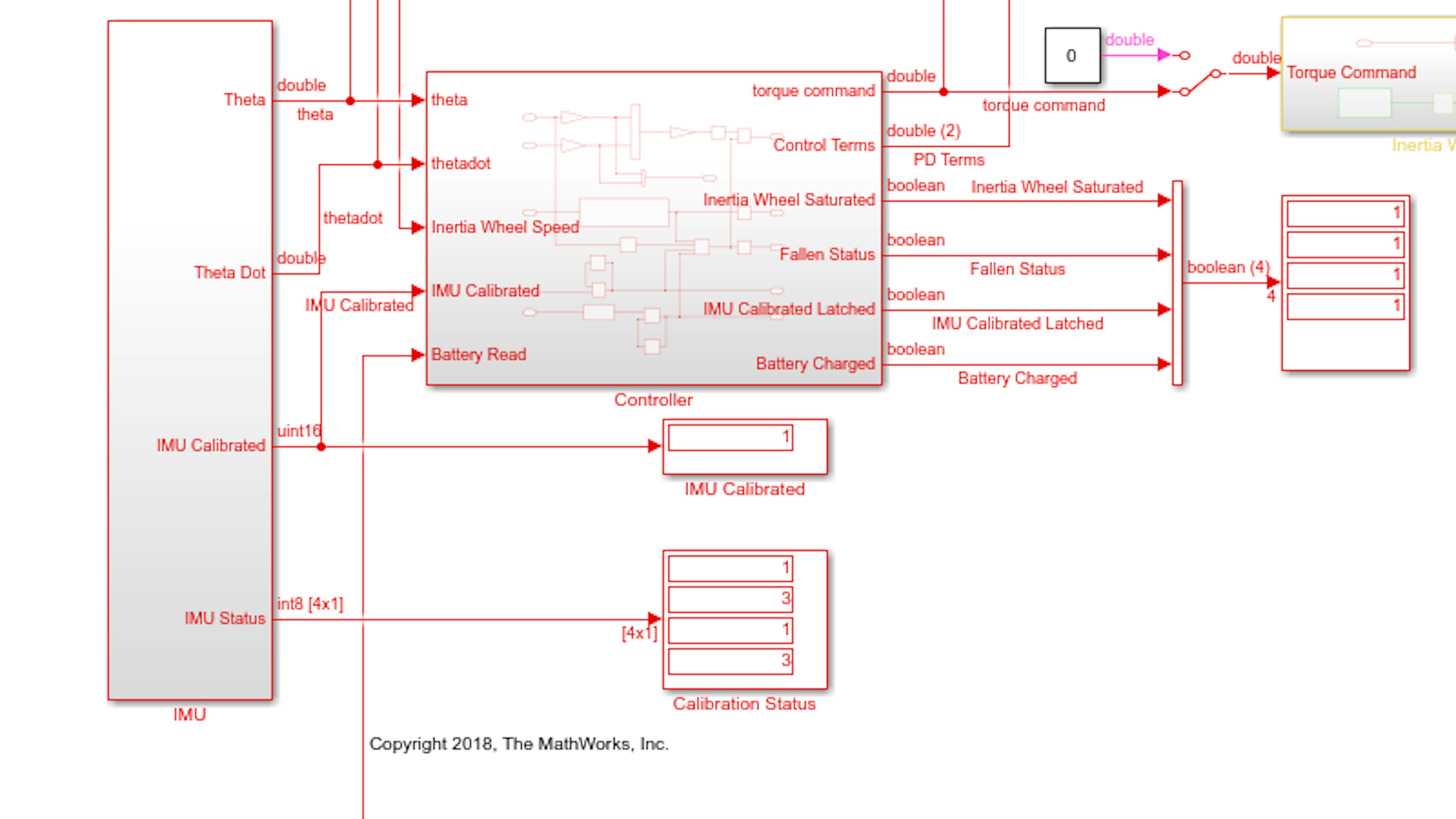
TESTING AND REFINING THE CONTROLLER ALGORITHM ON MKR1000
Next, let’s attempt to balance the motorcycle using the inertia wheel. Initially, you will need to shift the center of mass of the motorcycle so that the center of mass point is directly above the wheel-ground axis when the IMU measures θ to be zero. You can do this, for example, by shifting the position of the LiPo battery on the rear of the motorcycle.
With the inertia wheel motor disabled, try shifting the battery position from side to side. Run the model if it is not already running. Watch the Display block to ensure that the IMU is sufficiently calibrated:
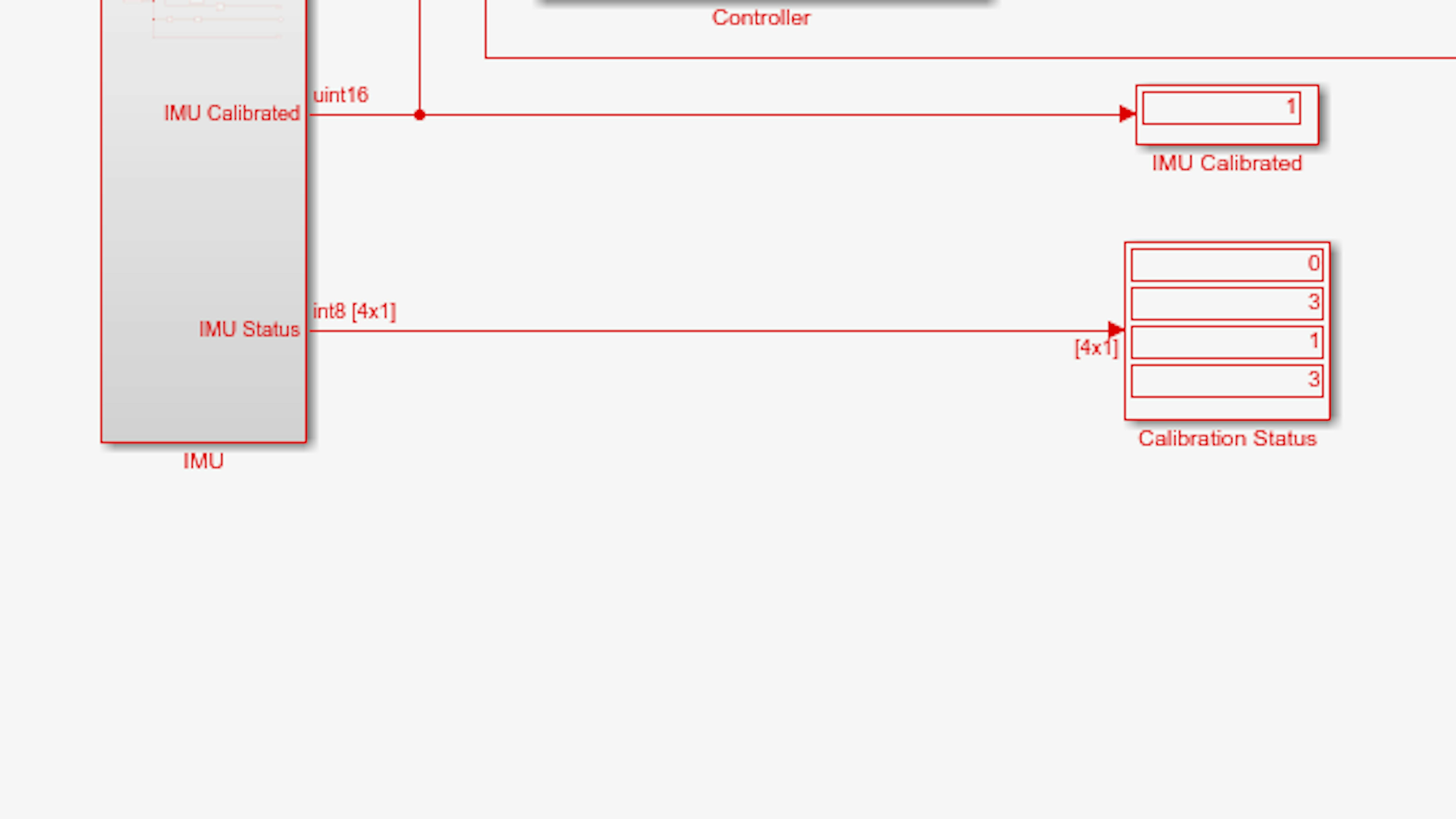
Hold the motorcycle vertically while observing the Scope window. Push the motorcycle back and forth a few degrees in each direction so that it moves freely across the balance point. Decrease the amplitude of the motion until you can identify the balance point within a few degrees:
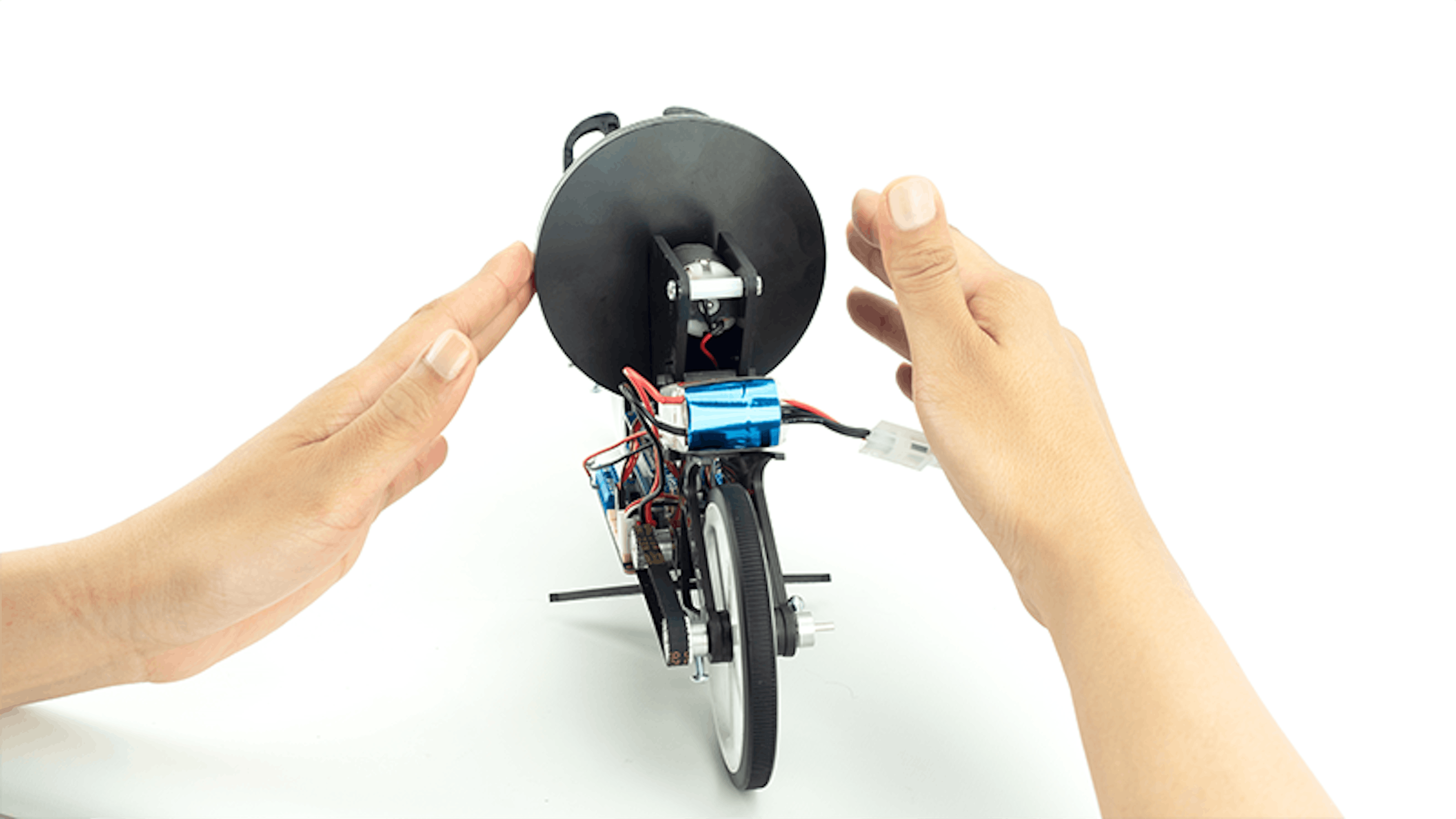
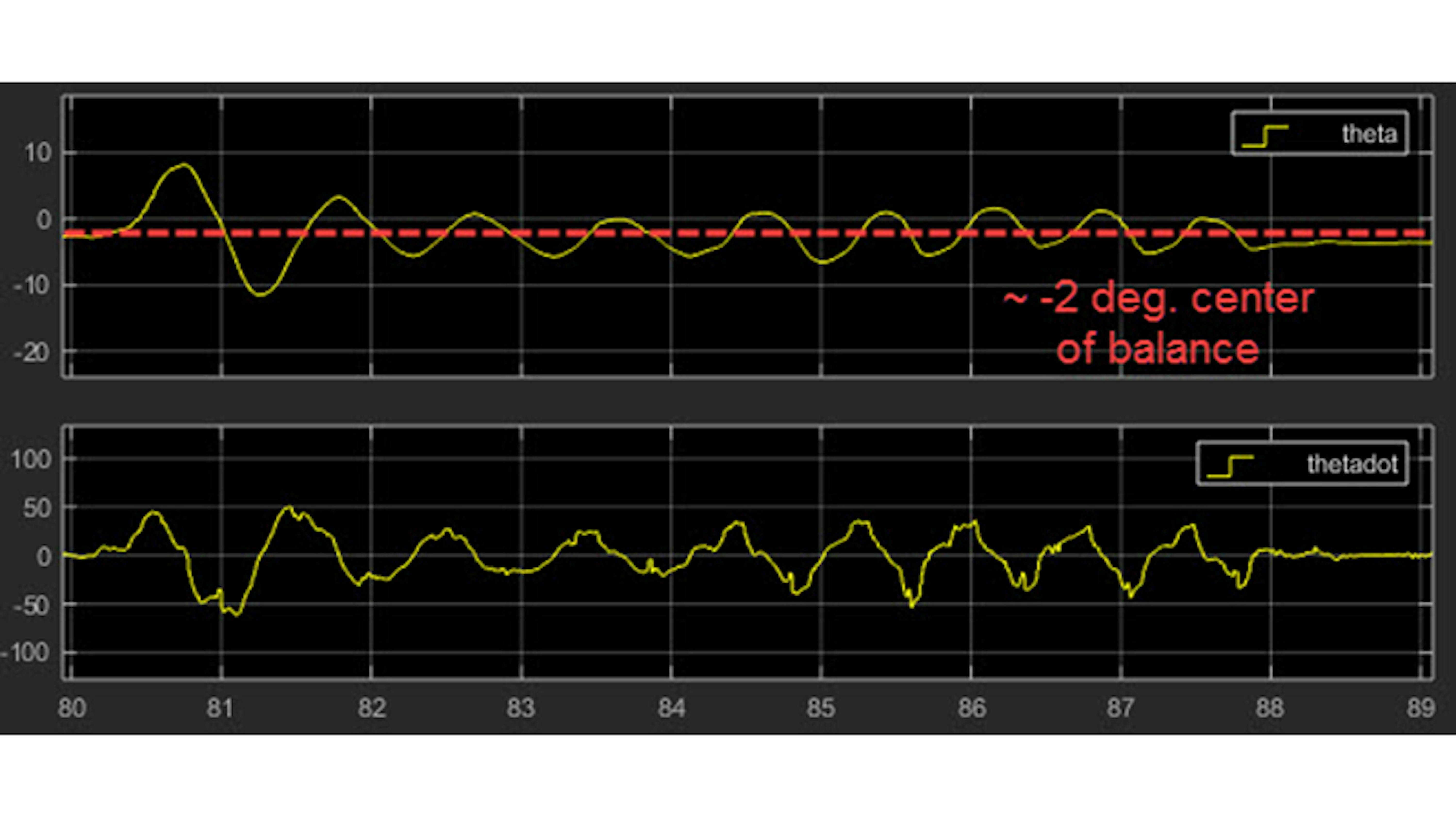
If you find that the center of balance has a negative bias, try shifting the battery to the right and repeating the test. If the center of balance has a positive bias, try shifting the battery to the left and repeating the test. Keep repeating until you get the center of balance within 1 degree of 0:
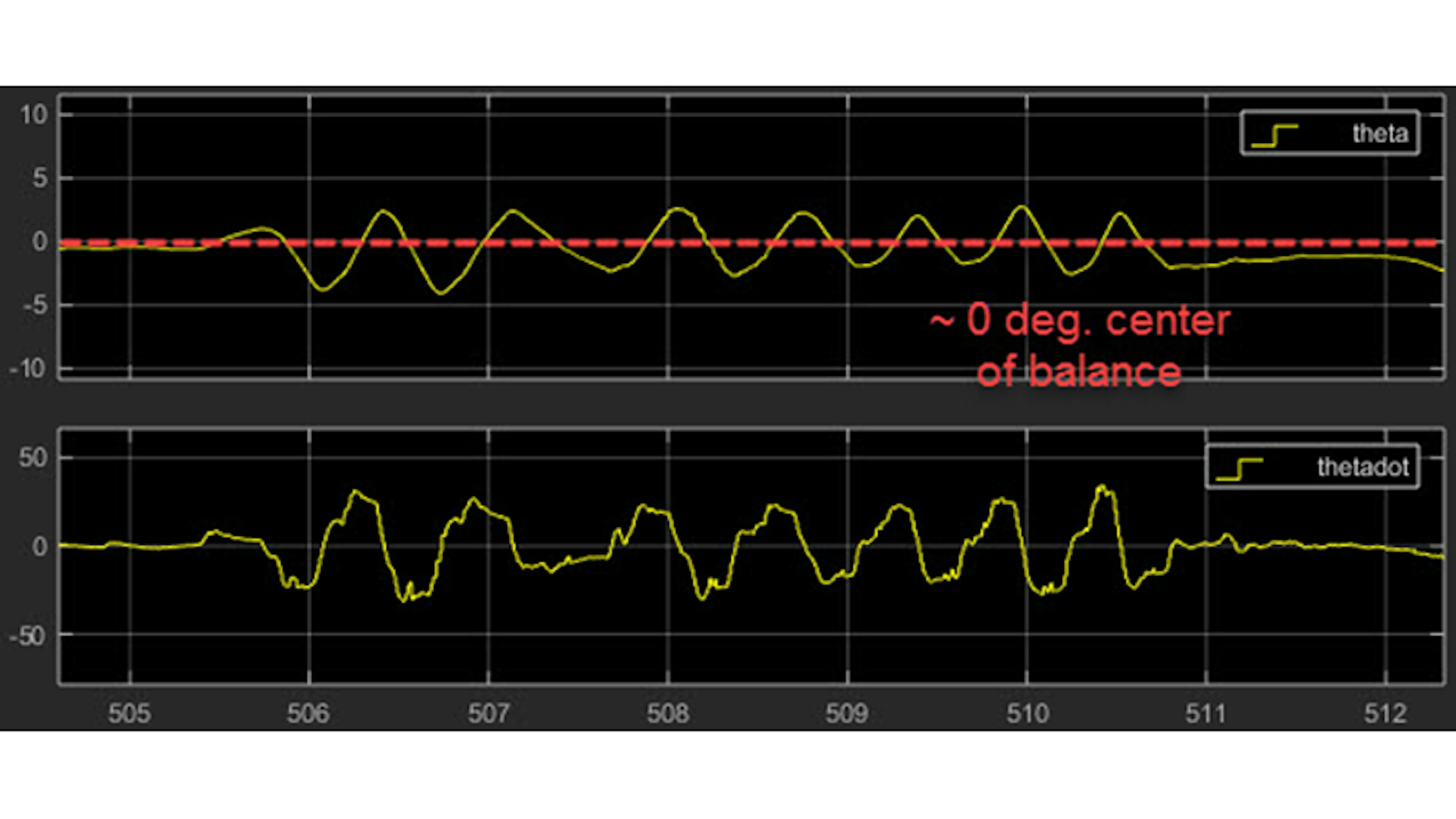
Note: If there is a more severe bias in your center of balance measurement (i.e. more than 4 degrees), make sure that the IMU shield is firmly pressed down onto the MKR1000 board and the MKR1000 board is pressed firmly down onto the motor carrier, which should then be flush with the bottom of the motorcycle frame. All three components should be visibly parallel to the ground surface:
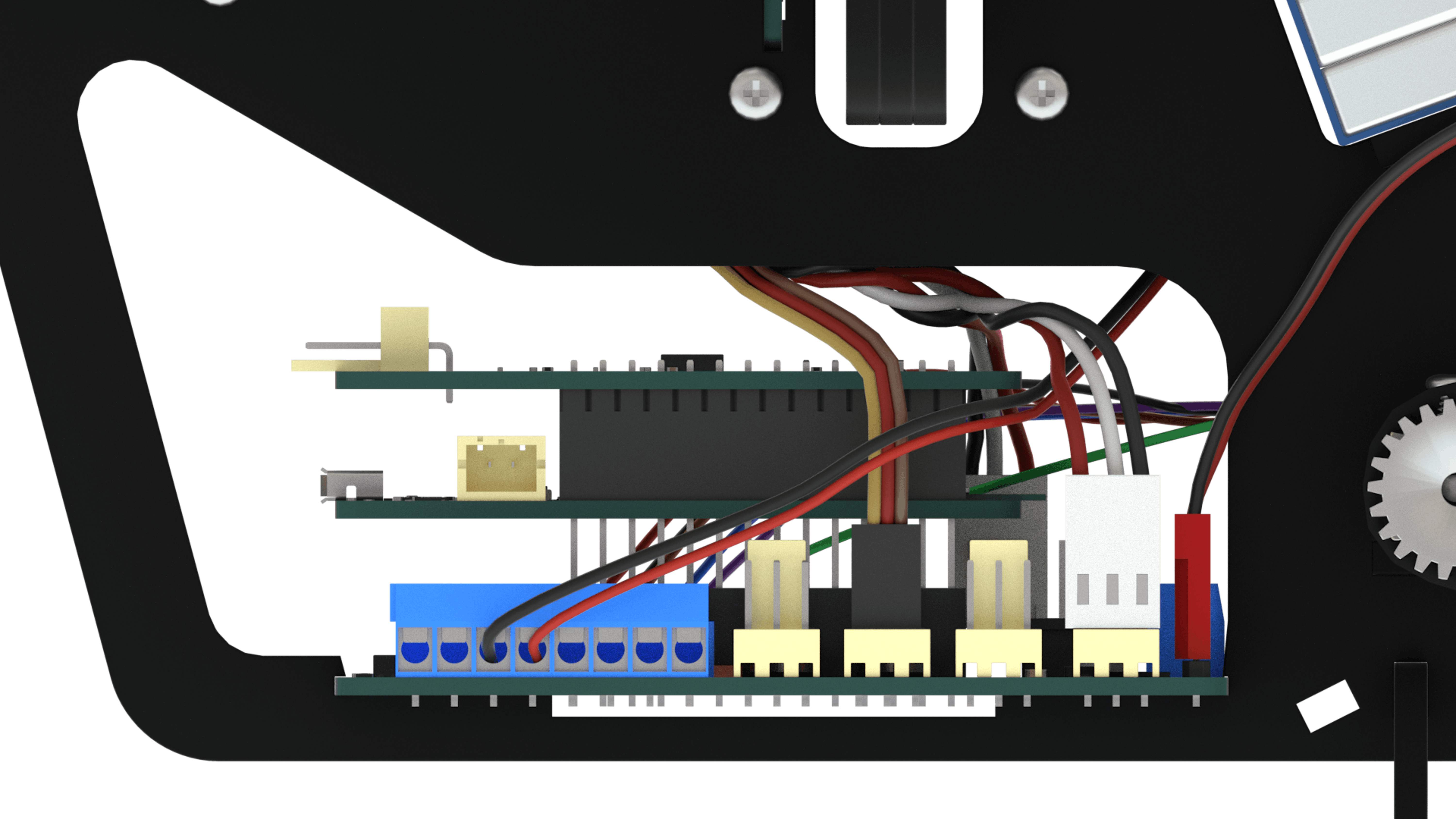
Set the center of balance
Sometimes sensors can have what we call Bias. In the case of IMU sensor, it could be because of the way it is mounted or that there is an external force on the motorcycle such as the USB cable pushing up against it. Let’s use the inertia wheel motor to fine tune the center of balance point and eliminate bias. While locking the inertia wheel with your fingers, enable the inertia wheel motor by using the Manual Switch block in the model window. The motor will begin to drive against your grip:
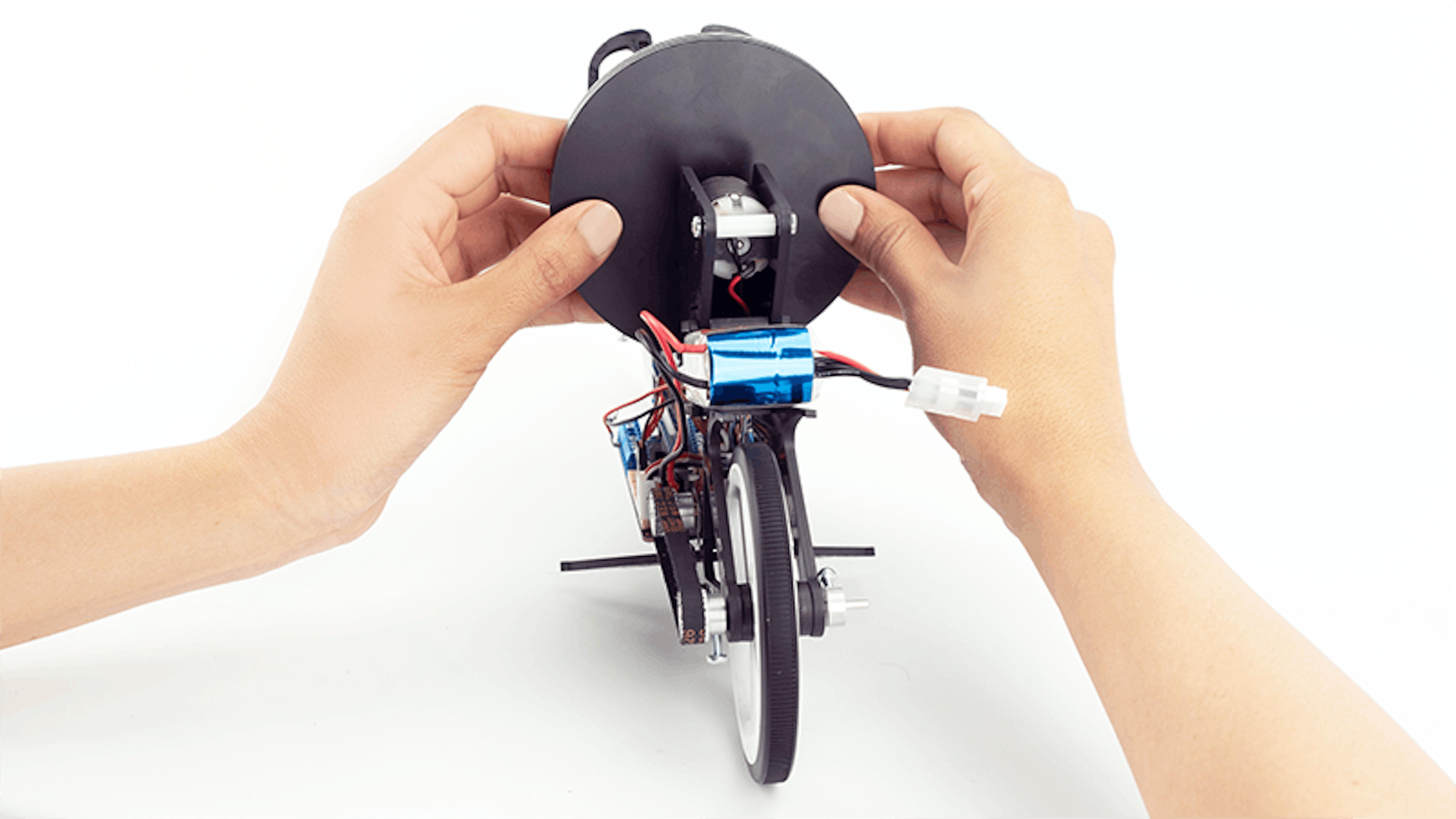
Adjust the lean angle until you find the angle at which the motor torque is zero (where it changes direction) Note this lean angle somewhere, this is the bias in your IMU.
Loosen your grip so that the inertia wheel is allowed to spin and the motorcycle is allowed to gently fall into either hand. See photo below:
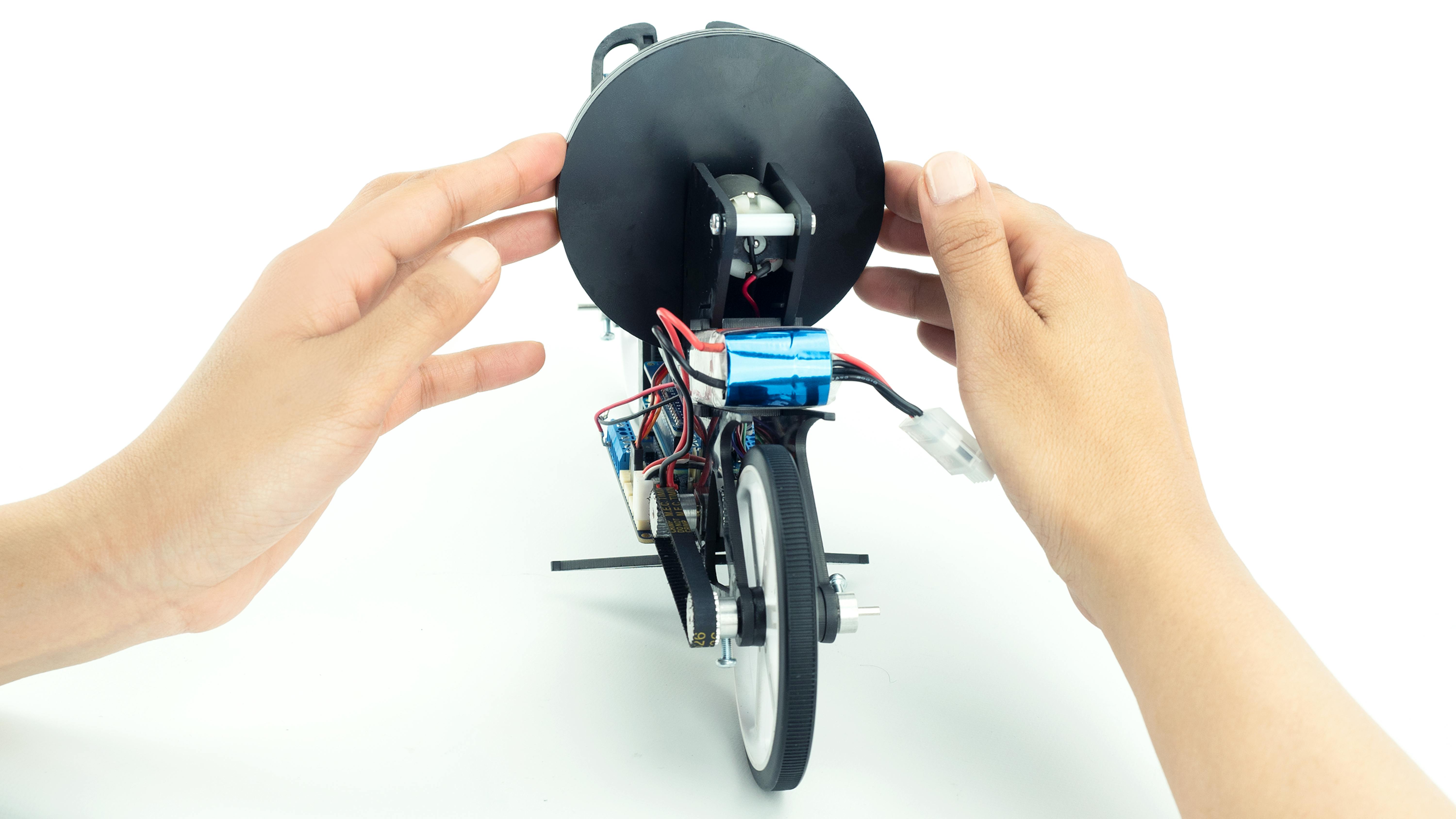
Repeat the last two steps several times until the hand the motor falls into becomes random. The average of these values is a good estimate of the bias.
Now let’s see how to adjust the bias in our model. Add a bias block (Simulink → Math Operations) into myNewMoto as shown below.
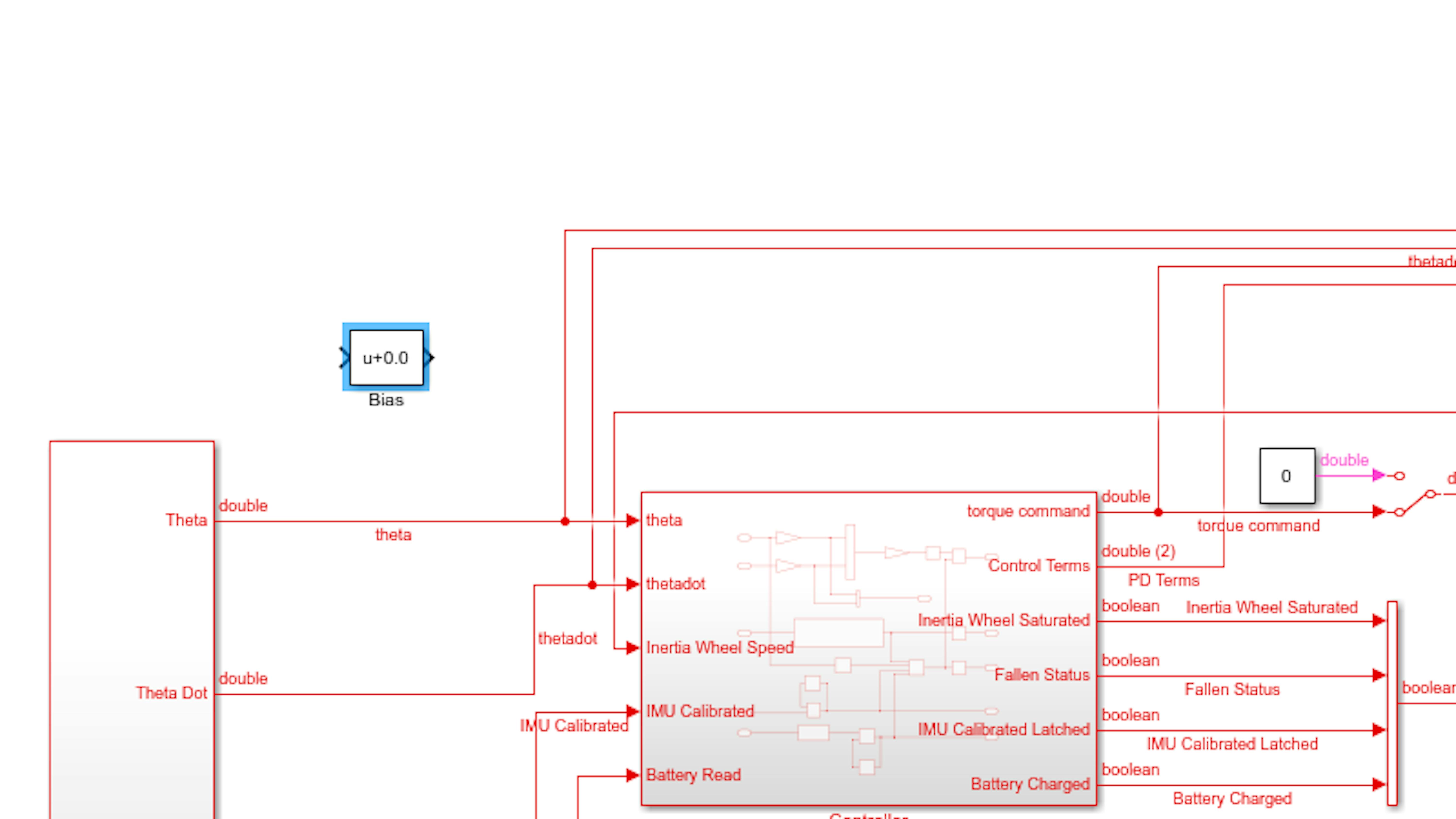
Drag the bias block onto the theta signal as shown below:
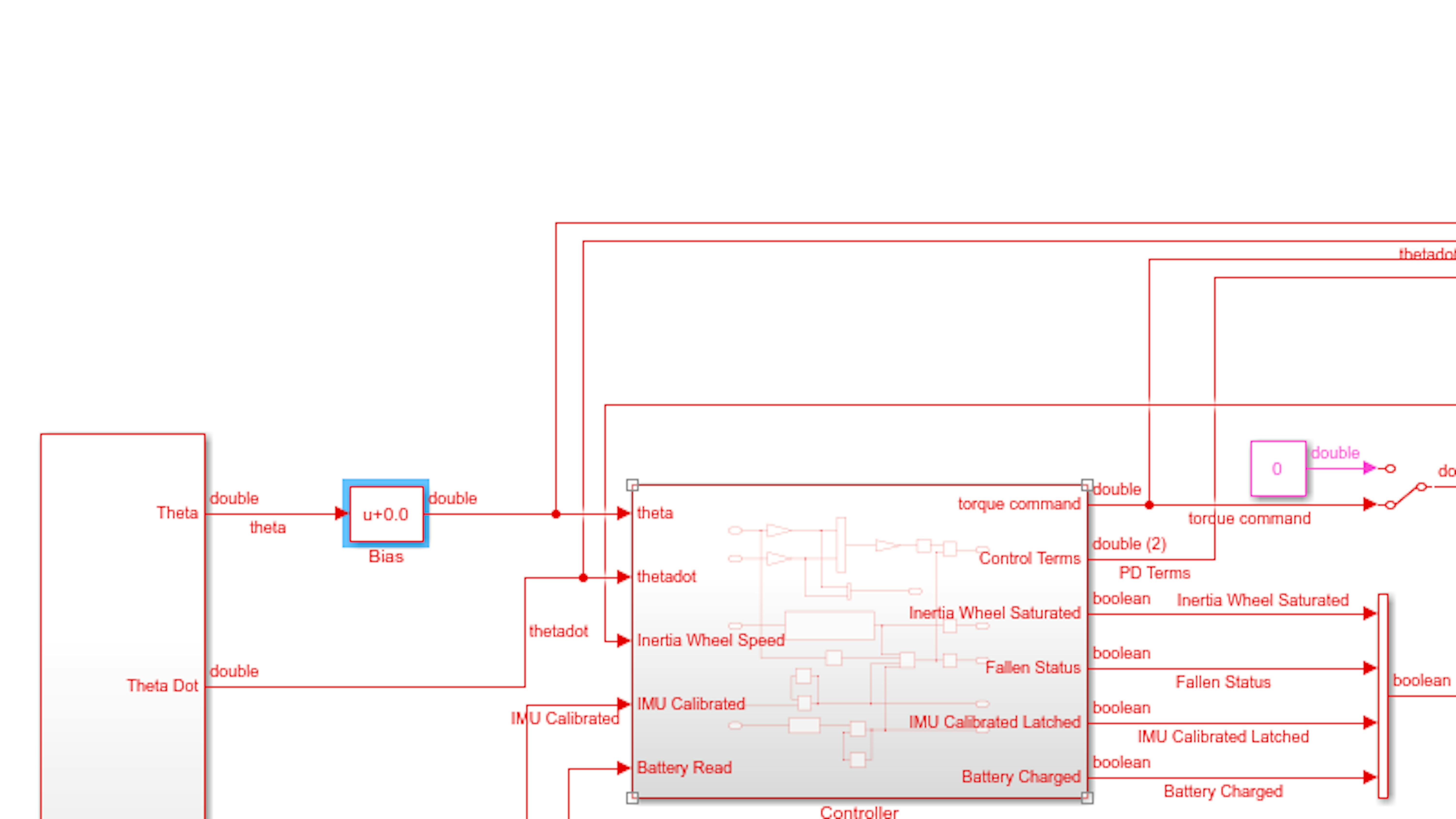
Add a Slider block from the Simulink → Dashboard library onto your model and double click on it.
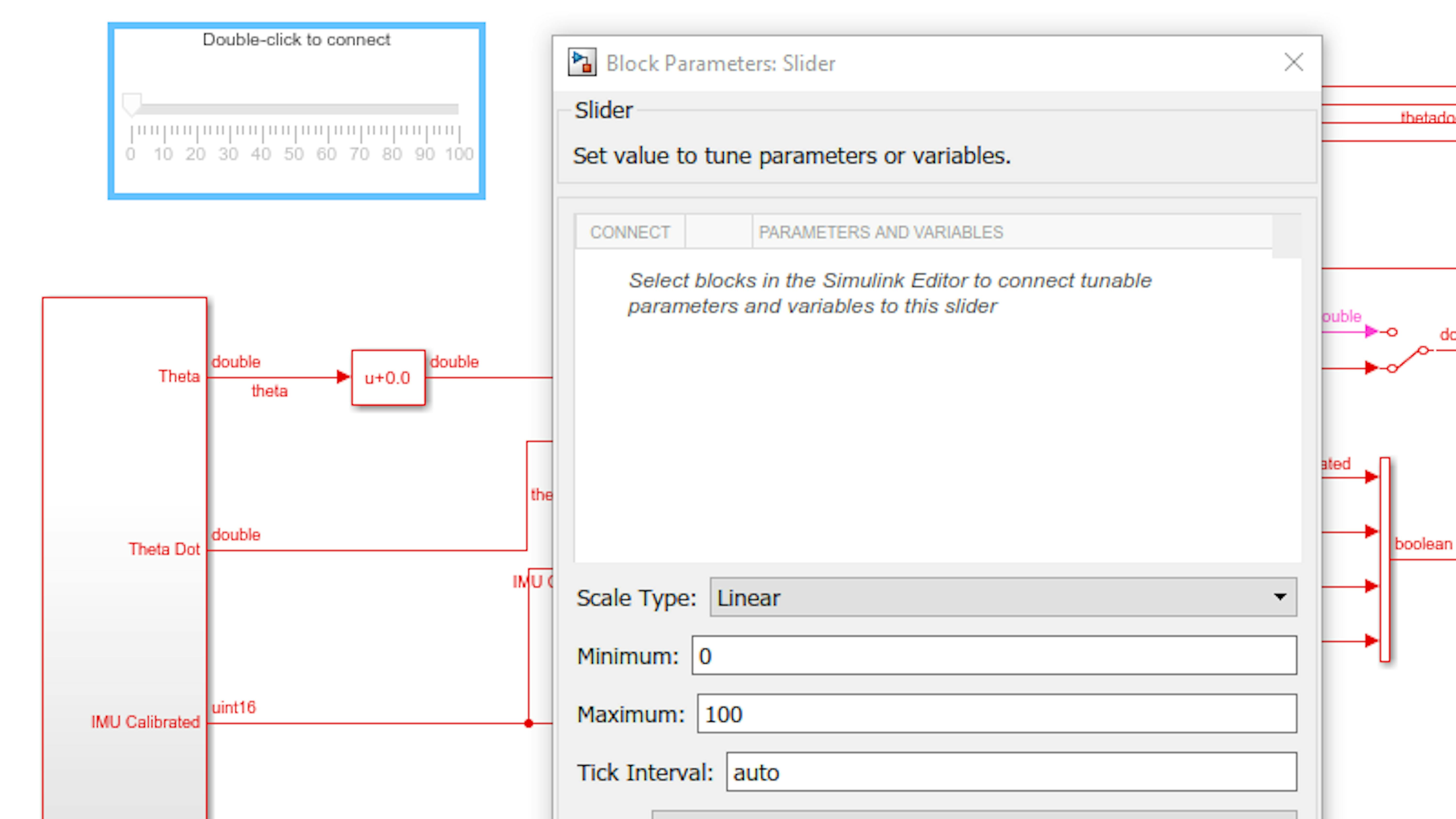
Select the bias block in the model and then check the circle inside the slider block and change the Minimum and Maximum value to -5 and 5 respectively.
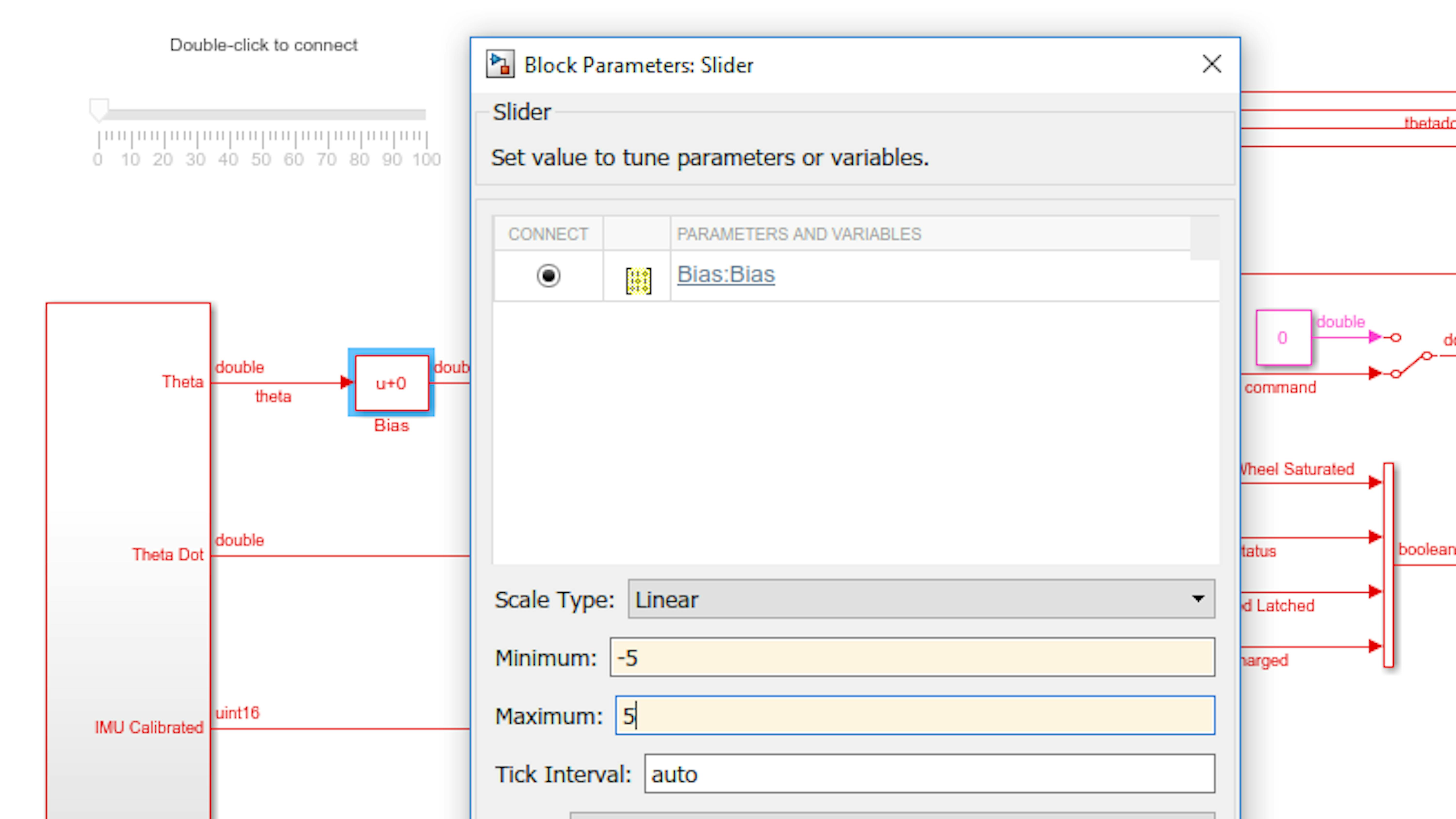
Here is what the finished model should look like:
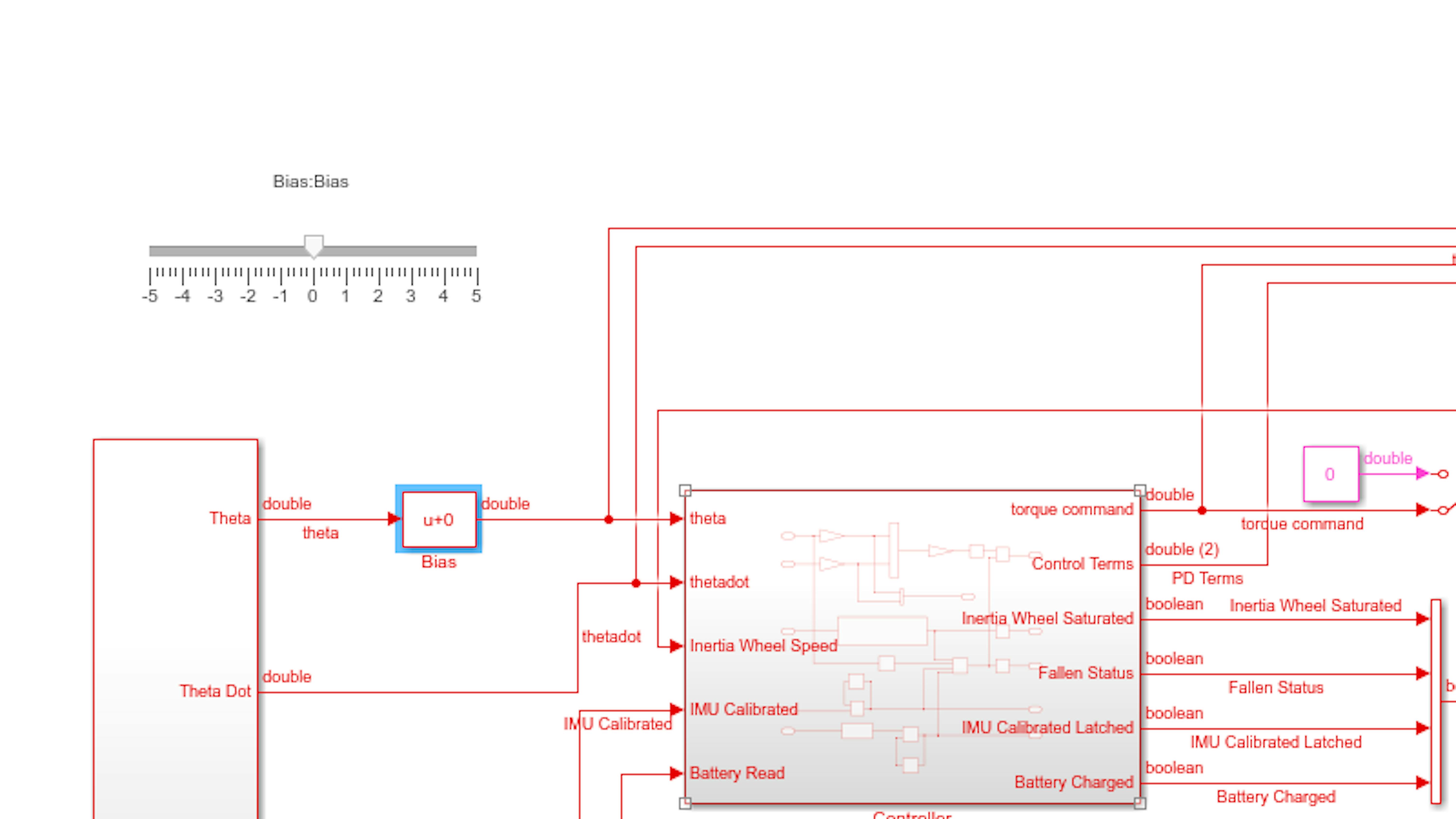
When you run the model in External mode, many of the block parameters, such as gains and constants, are tunable. This means that their value can be changed while the model is running on hardware. The bias is also a tunable parameter. You can double-click on any tunable block while the model is running and enter a new parameter value. The new value takes effect when you click Apply or OK in the block dialog window. Moving the slider has the same effect as changing the value of bias inside the block and clicking on Apply.
Run this model and eliminate the bias value you obtained so that your controller can balance for at least 10 seconds.
Note: While doing this test, if you notice that the inertia wheel saturates too often without the motor getting hot feel free to increase the Saturation limit to 6000 as shown below.
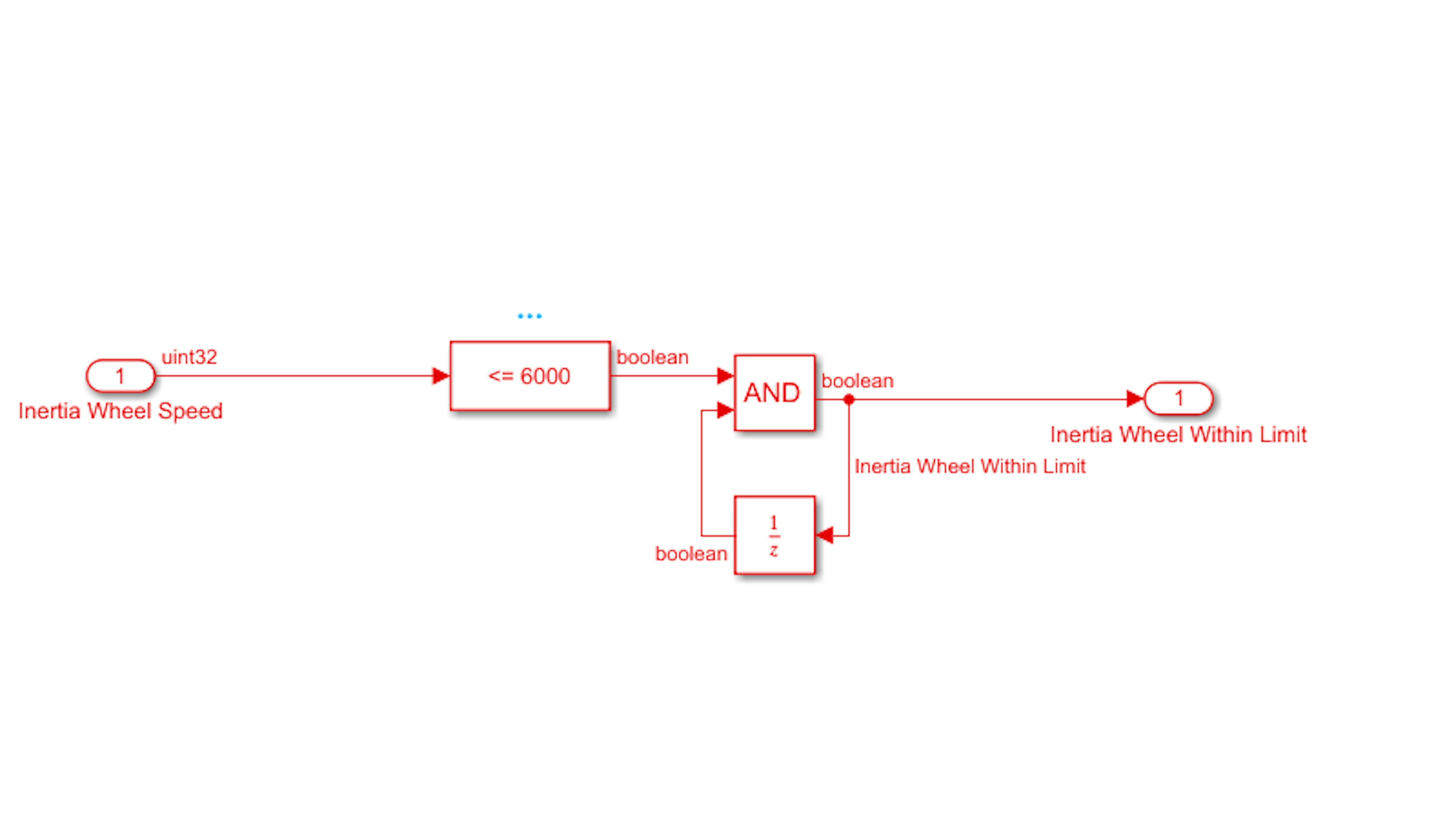
Tune the Controller gains
Now it is time to tune the control gains to find the optimal control law for balancing the motorcycle. There are many approaches to systematic PID controller tuning in the engineering literature. Similarly, there are many software tools available, including Simulink Control Design, that attempt to determine the optimal control gains by observing the state errors over time and characterizing the behavior of the system under control. For the initial tuning of the controller, it is helpful to attempt the tuning manually to get intuition for the system behavior and the effect of each control gain.
In most PID tuning methodologies the I and D gains are considered proportional to the P gain, and one should not adjust P without making equivalent proportional changes to I and D simultaneously. Otherwise, it would be difficult to assess the effect of a change in P alone.
What we have is a pretty aggressive controller as you can see that the P and D terms are in similar magnitudes. Let’s change the value of Kd and see how the motorcycle behaves while holding Kp gain constant.
Confirm that the P and D gains are still set to 25 and 4, respectively, and the Gain is still set to 2e-2 (or Kp =33.33, Kd = 5.33 and Gain = 1.5e-2 for 6V motors):
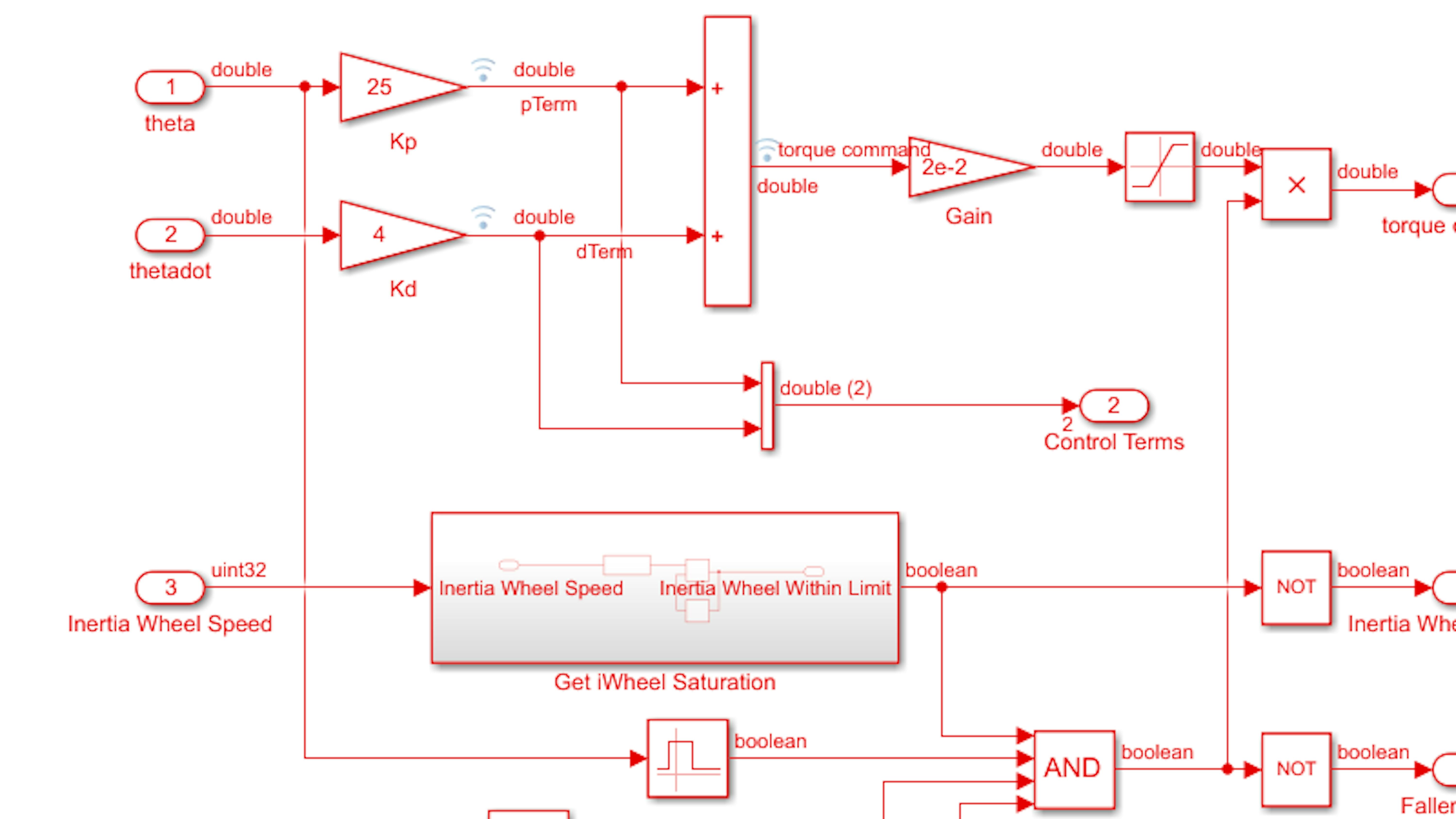
Now, make sure the inertia wheel motor is disabled and run the model. Calibrate the IMU. With the inertia wheel motor on the center-of-balance check as before, make sure the lean angle oscillates roughly around 0. Adjust the bias value as needed:

Hold the inertia wheel motor and enable it. Release the motorcycle from the vertical position and attempt to balance it. You might also observe theta dot has a noise about the balance point (meaning that even though the motorcycle is not osciallating this value is changing a lot):
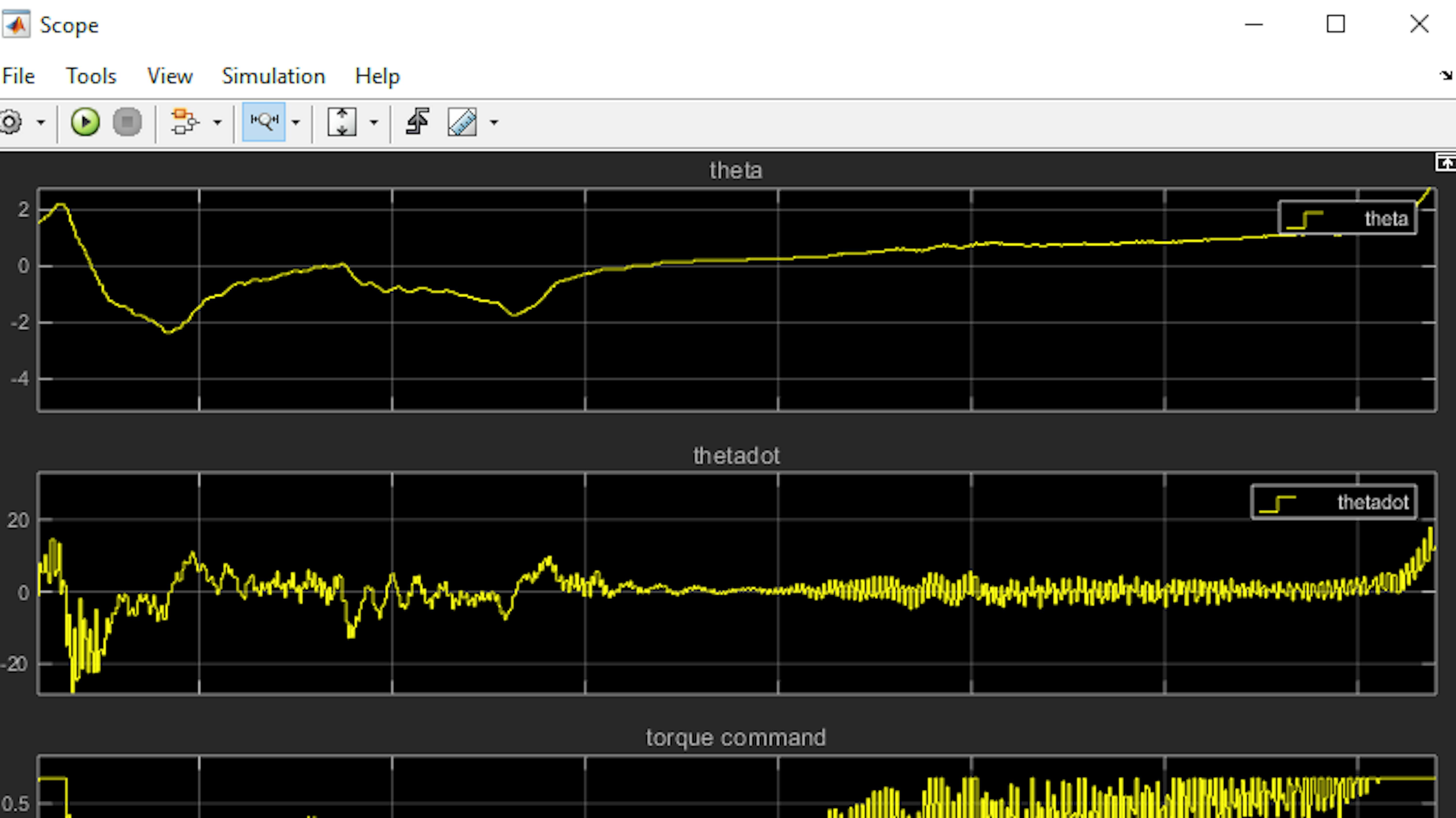
Now, let’s see if you can improve stability and reduce oscillations.
Let us reduce the influence that D gain has on the control by reducing its value to 0.4. Change the Kd gain as the model is still running on the hardware and observe the change in theta.
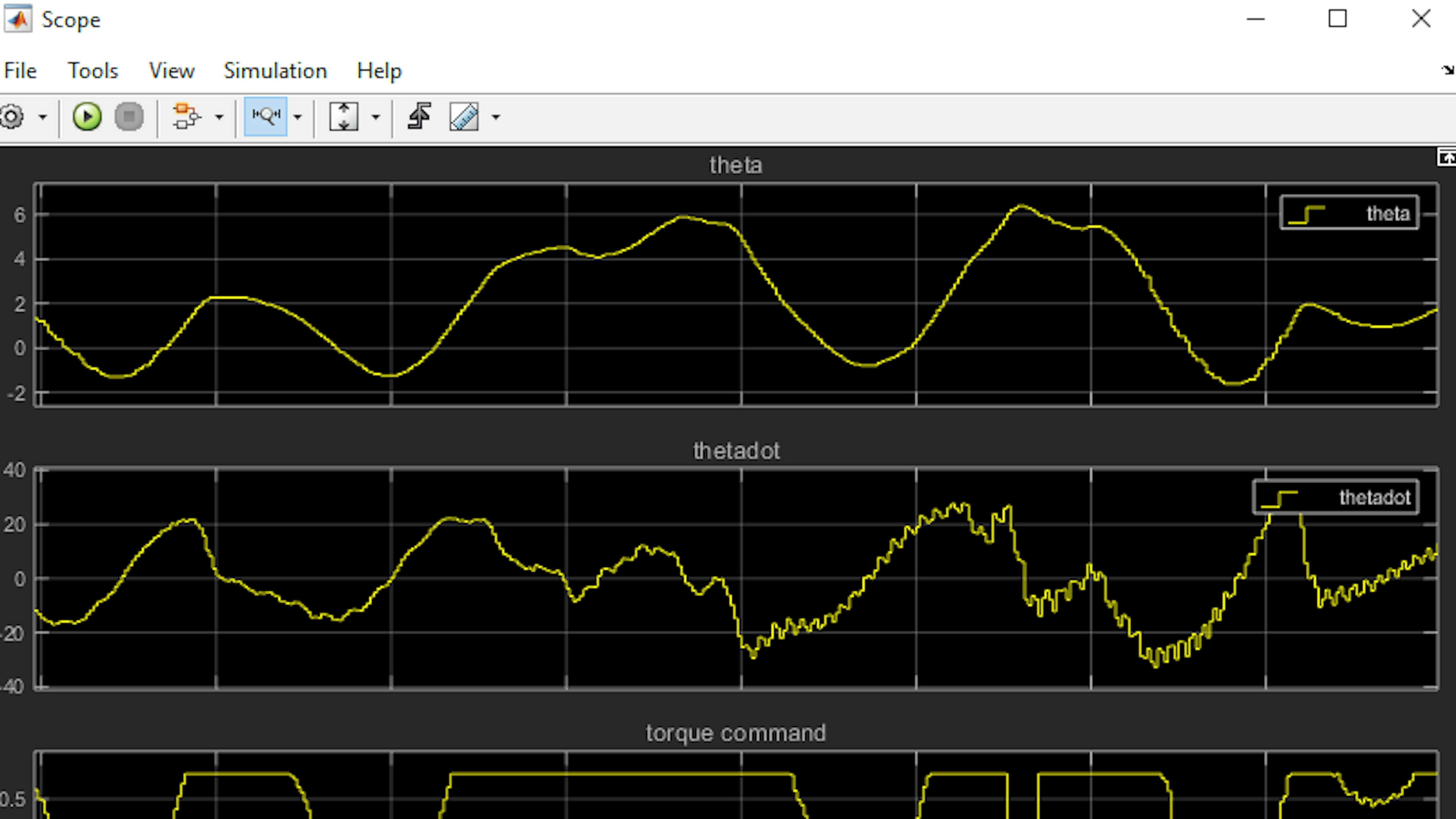
You will definitely notice that the theta is more oscillatory because of this, which suggests that the only way to go for Kd gain is up. Play around with the Kp and Kd values to get a good controller that can balance at least for 20 seconds. Remember, if your motorcycle is experiencing a steady state error, you can increase Kp to eliminate it if you are increasing Kd, Kp needs to be increased as well.
Moving forward, let’s consider your baseline controller tuning as follows:
When you are finished tuning your PD controller, return the controller gains to the values above before proceeding to the next exercise.
Deploying the algorithm to the motorcycle
So far, we have seen how to run the balancing algorithm on the hardware while the motorcycle is still connected to the PC via USB. To run your well-tuned control algorithm standalone on the hardware, click the deploy to hardware button and watch your motorcycle balance in place even after disconnecting the USB cable. Remember to power the Motor Carrier ON after disconnecting.
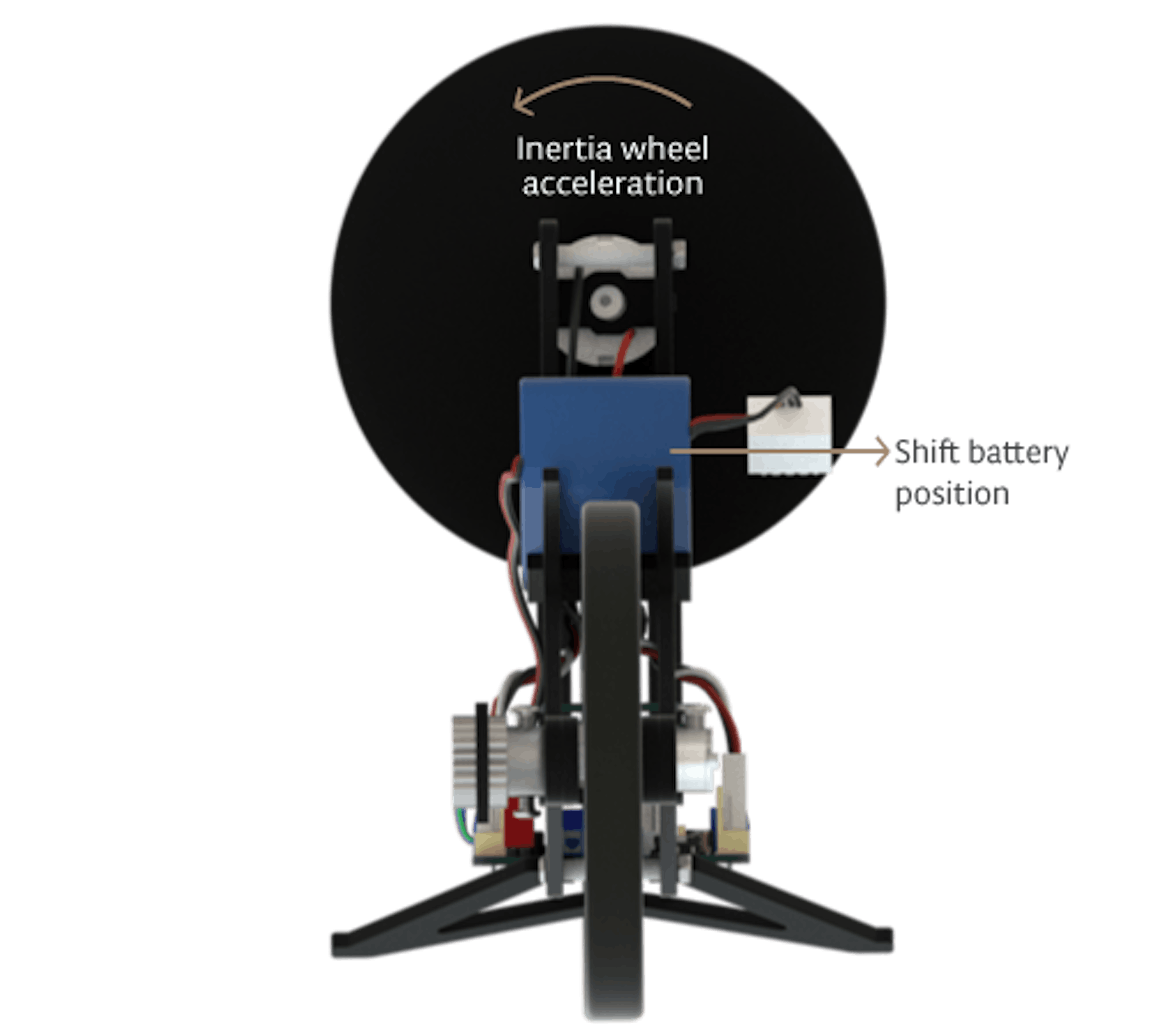
LEARN BY DOING
In this chapter, you have integrated the inertia wheel motor, the IMU sensor, and the tachometer into the main system model so that they correctly interface with the PID control algorithm. You then added safety features to minimize the risk of damaging the hardware. Finally, you tested the balance control algorithm on the real hardware and fine-tuned the control algorithm and its PD gains to achieve balance in place.
To explore further, try adding -
- saturation to the D term to reduce the impact of oscillatory theta dot signal.
- various perturbations to the motorcycle while it is balancing in place. For instance, if you have a fan (or a windy climate), try exposing the motorcycle to wind from various directions.
- a non-level or vibrating surface.
How well does the controller balance the motorcycle under varying external circumstances?
Another challenge that you can try is adding another safety feature that disables the inertia wheel when the torque command has saturated to 0.7 or -0.7 for a specified amount of time. You should keep in mind that it is acceptable for the inertia wheel motor torque to hit the saturation limits occasionally, but it should not stay at these value for a long time or hit those values very frequently. It is your choice how you construct the enable/disable logic with respect to the inertia wheel motor’s torque command. Ultimately, find an algorithm that balances the safety of shutting off the motor due to severe saturation behavior against the practicality of keeping the motor running under reasonably safe circumstances (such as very sporadic and short saturations).
EXERCISE 4:
6.4 Balancing with straight motion
In this exercise, you will balance the motorcycle as it moves in a straight line forward or backward. To do this, you will need the algorithm to run on the MKR1000 while not connected to your computer’s USB port. Technically you can do this now, but once you disconnect the MKR1000 from the computer, you have no knowledge of the system statuses, the control terms, or the angle. Furthermore, you cannot control system modes via manual switches in the Simulink model. Therefore, you will implement a Wi-Fi connection between the motorcycle and the computer so that you can wirelessly observe the motorcycle’s status and signals on your computer without the physical connection. Then, you will introduce the rear wheel component, first, in isolation, and then into the motorcycle model that you have worked on in previous exercises. You will then run the control algorithm on the motorcycle while controlling the rear wheel via Wi-Fi and observing its signals remotely.
In this exercise, you will learn how to do the following:
- Control and monitor the motorcycle remotely via Wi-Fi
- Understand the capabilities and relevant specifications for the rear wheel DC gear motor and the rotary encoder.
- Test and integrate the rear wheel motor to enable forward and backward motion of the motorcycle
- Balance the motorcycle while moving forward, backward, and in place.
CONTROLLING AND MONITORING MOTORCYCLE VIA WI-FI
Let’s begin by configuring the system model to run the controller algorithm remotely. To proceed with the motorcycle project from this point, you will need access to a Wi-Fi network. The network must be open (no password) or with WEP or WPA encryption. The network must not require additional credentials beyond the WEP or WPA security (like captive portals requiring interaction with a website, for instance). If such a network is not available, you can create a Wi-Fi hotspot on your cellular phone. You can then connect your computer to your phone’s Wi-Fi network. See your phone’s user guide for instructions on setting up a Wi-Fi hotspot.
Connect your computer to a Wi-Fi network with the above requirements.
Open myNewMoto.slx:
>> myNewMotoNote: If myNewMoto.slx is unavailable or incomplete, use motoSys2_balance.slx instead and save it as myNewMoto.slx.
Open Configuration Parameters and navigate to the Hardware Implementation pane. Expand Target hardware resources by clicking on it and then click WiFi properties. Enter your network credentials:
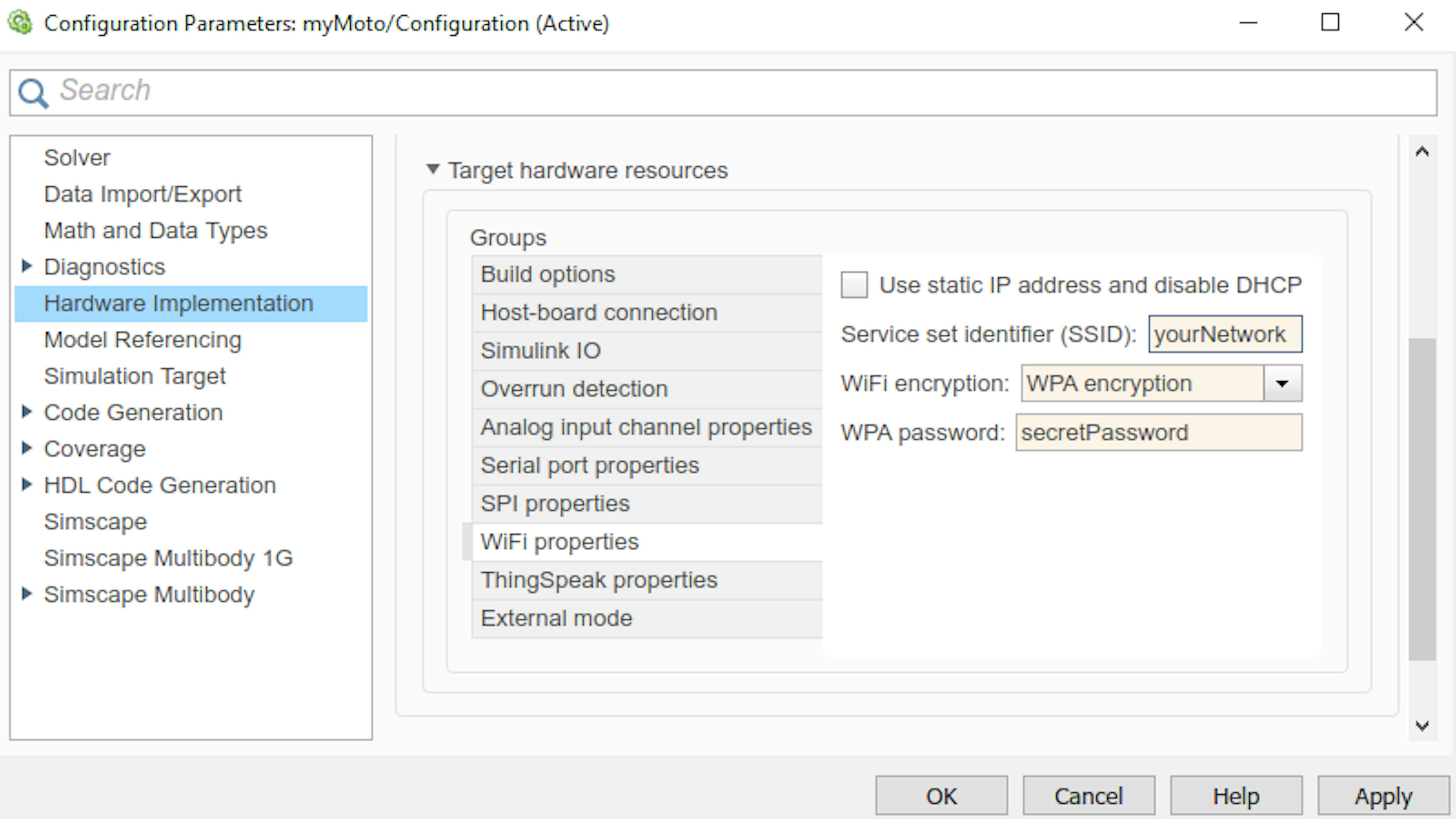
Next, click External mode and set the Communication interface to WiFi:
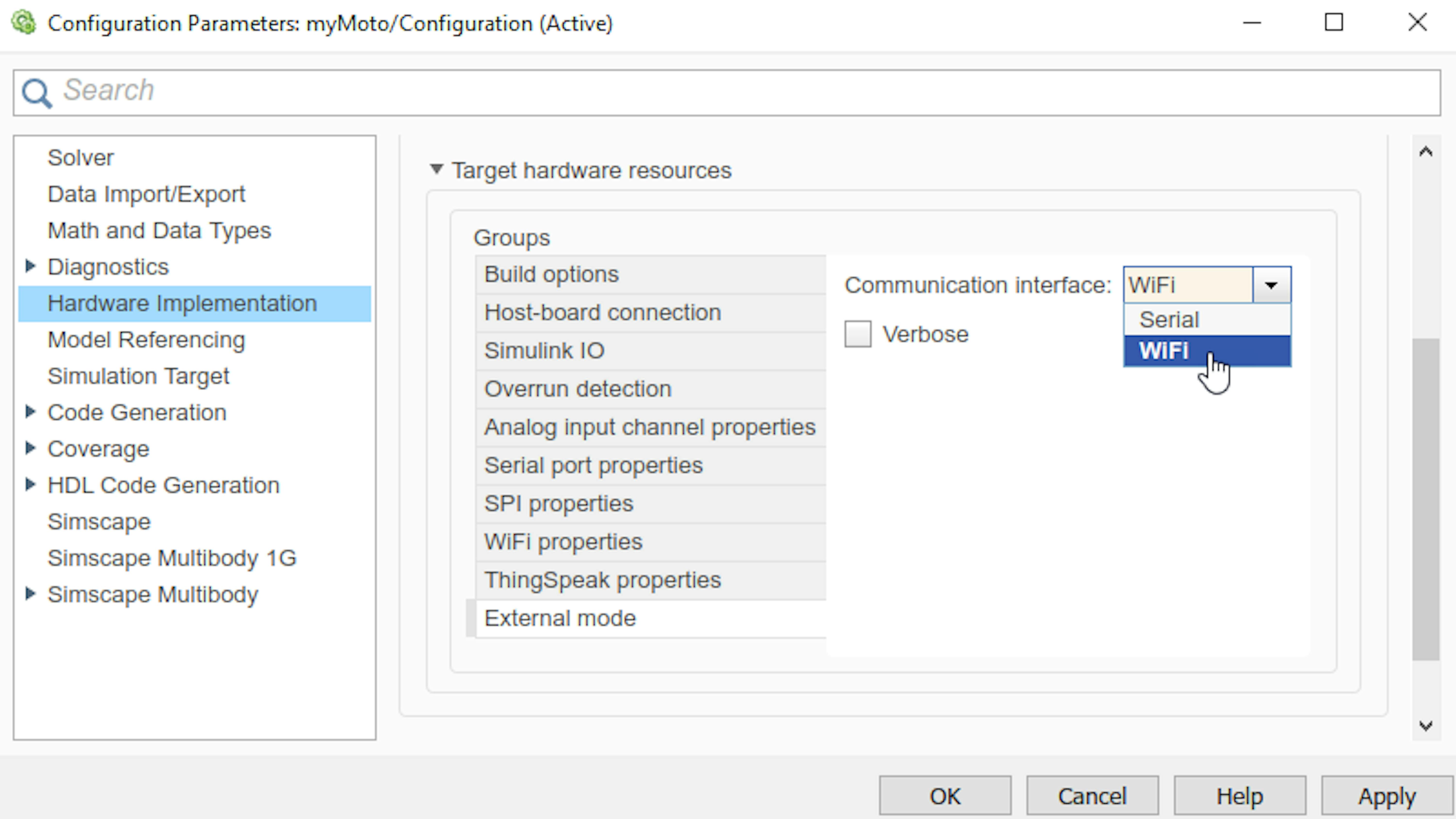
Click OK.
Run the model.
The build process will take a bit longer than usual since Simulink needs to scan your wireless network and find an available IP address for the MKR1000 board.
Once the model is running, disconnect the USB cable from your computer. Ensure that the model continues to run without errors. Examine the Scope window and make sure you are still streaming signal data. Calibrate the motor and balance the motorcycle as you did in the previous section:
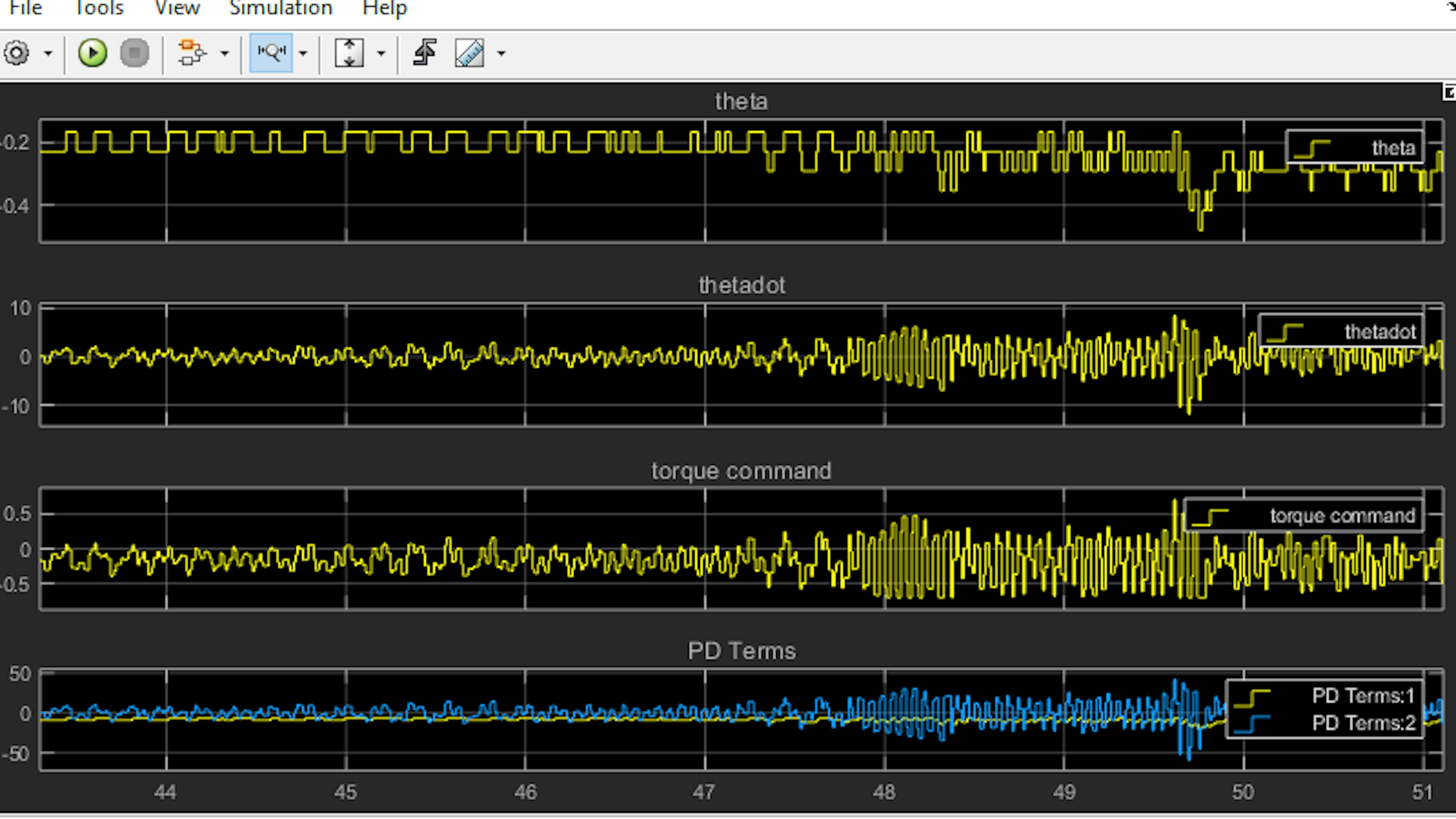
Try enabling and disabling the inertia wheel. How fast does the motorcycle respond to your commands?
Provided your Wi-Fi connection is stable and not too heavily trafficked with other data, you should observe a nearly instantaneous response between flipping the manual switch in the model and the inertia wheel motor becoming enabled.
Stop the model.
DRIVING REAR WHEEL
Now, let’s look at the rear wheel motor. The rear wheel is driven by a 100:1 gearbox DC motor. See the hardware specifications. You will integrate this motor into Simulink in much the same way you did for the inertia wheel motor.
While you are testing the rear wheel in isolation, it is useful to have the rear wheel elevated from your working surface so that the motorcycle does not drive away! To do this, remove the kickstand from the motorcycle and reconnect it in the vertical configuration:


Reconnect the USB cable to your computer.
Open the following Simulink model:
>> drive0_startSave the model as myDrive.slx.
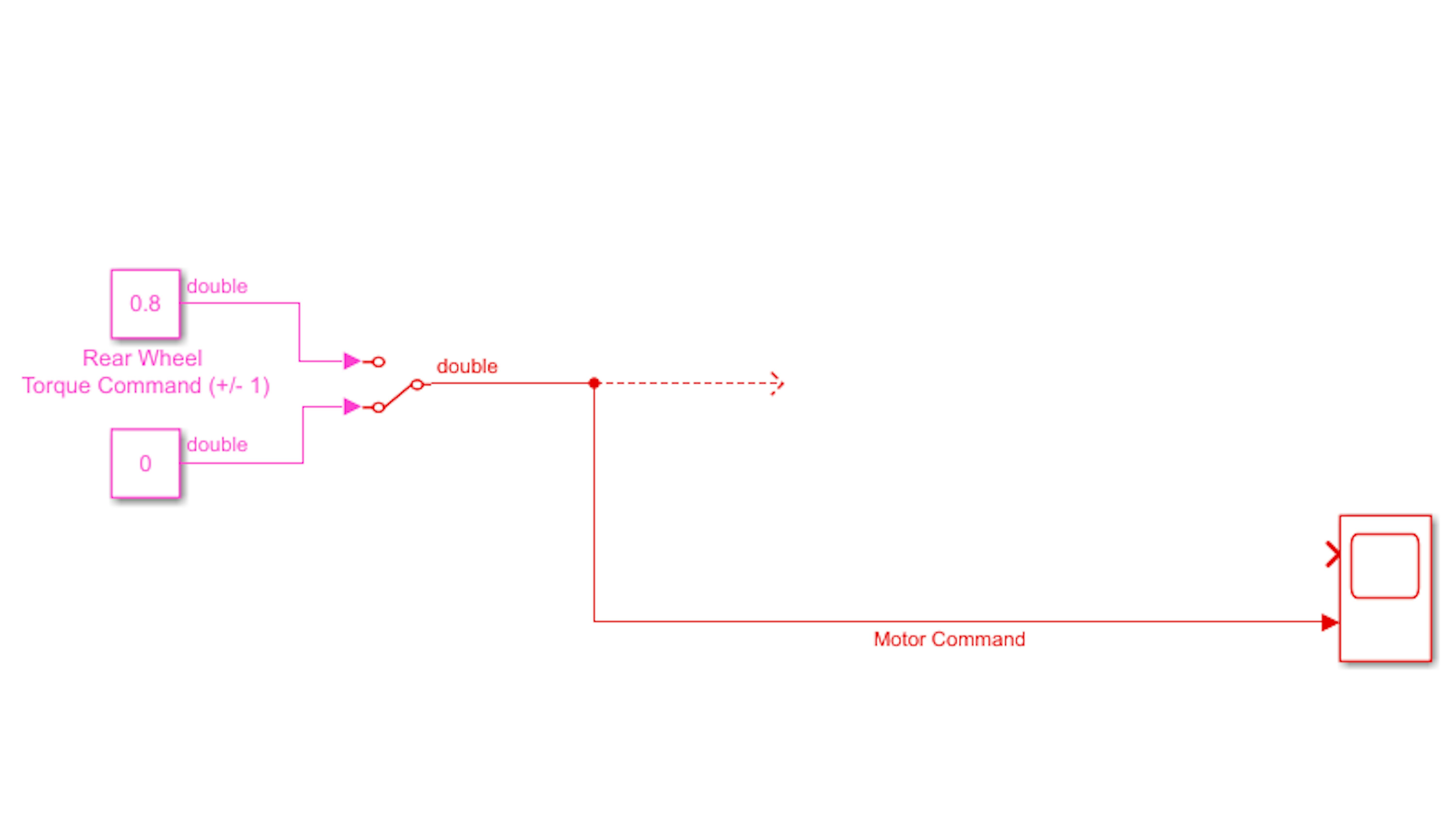
In this model, you will command the rear wheel speed as a fractional duty cycle with positive values indicating forward motion. A manual switch is provided to enable or disable the rear wheel motor.
Now, go back to myNewMoto.slx and copy the Inertia Wheel subsystem. Paste the subsystem into myDrive.slx and change the label as shown:
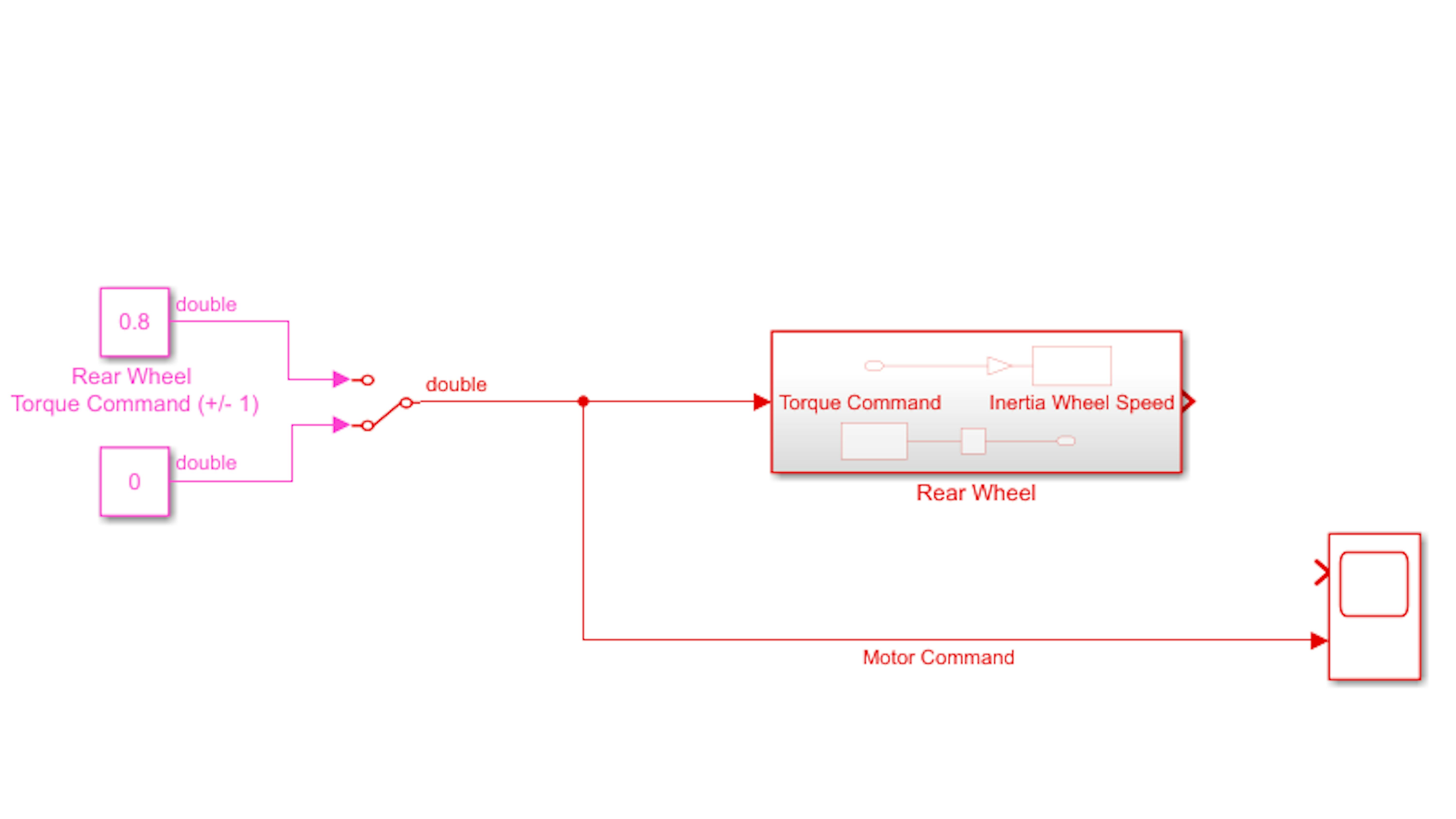
Examine the motorcycle to see how the rear wheel is connected to the motor carrier. Note the motor port label:
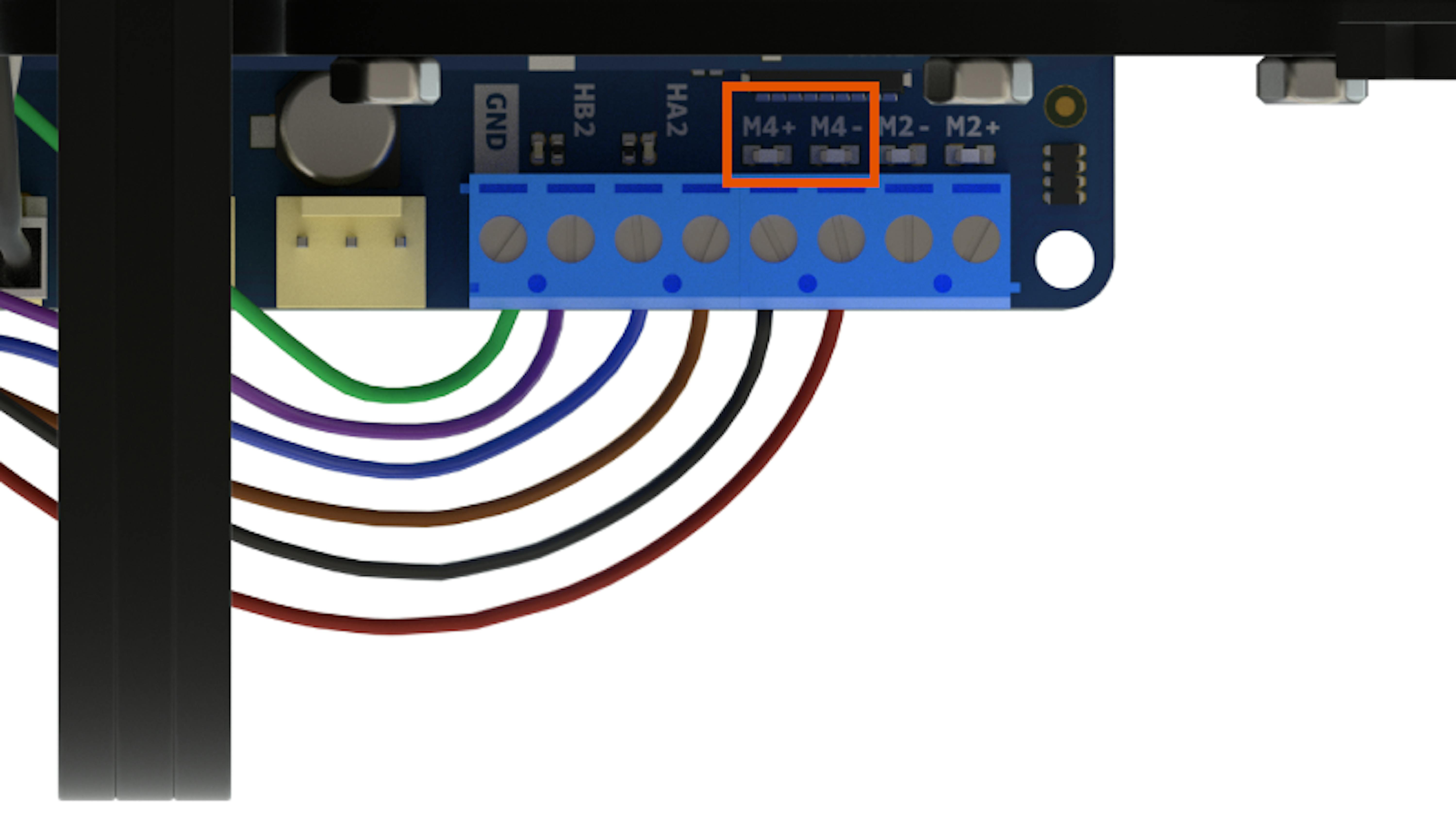
Access the Rear Wheel subsystem and then double-click the M3M4DCMotors block. Set Motor port to match the motor port label on your motor carrier and then click on Apply and OK:
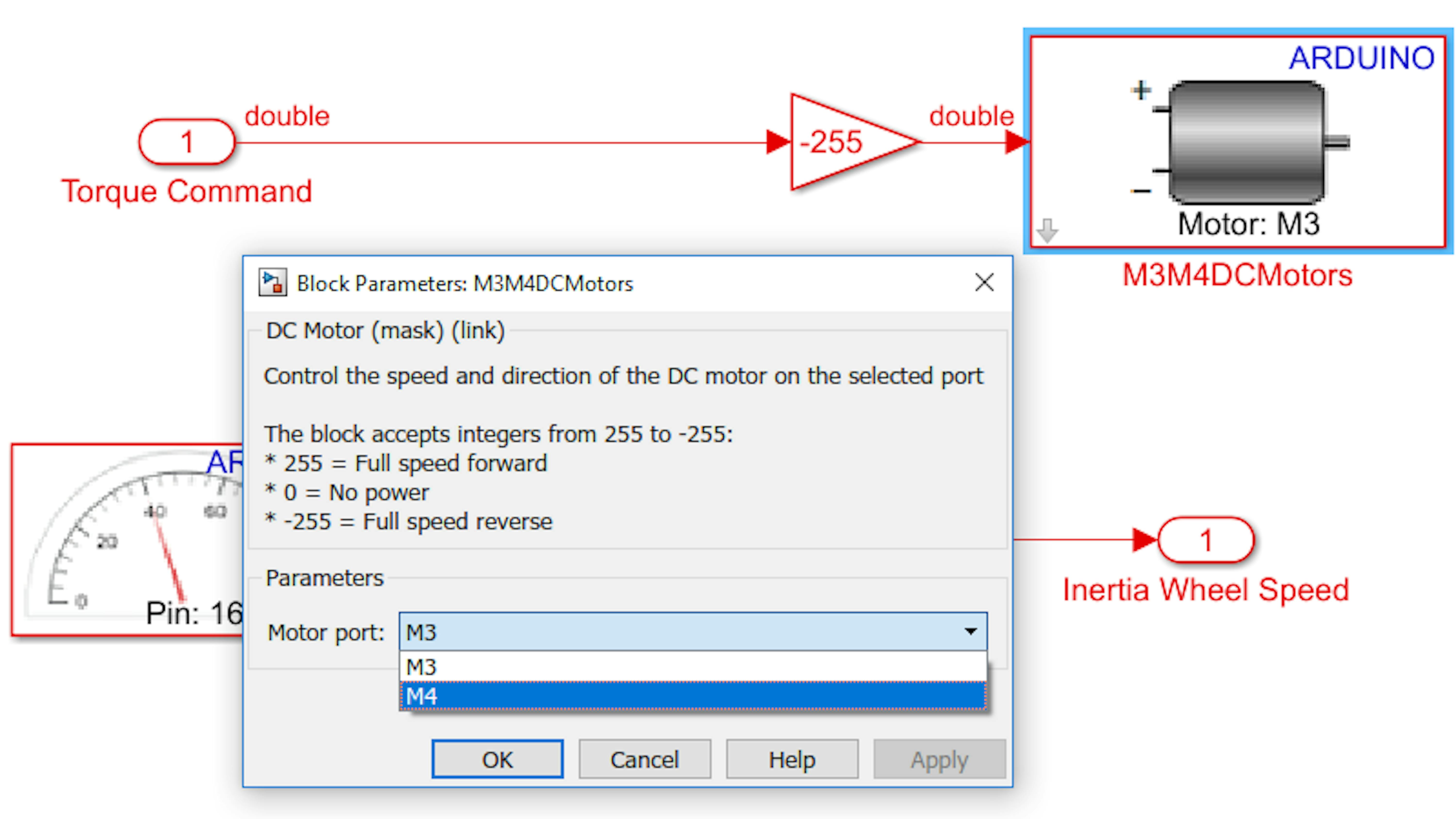
Delete the bottom portion of the subsystem, consisting of the Tachometer block, the Rate Transition block, and the Inertia Wheel Speed outport. You will later replace this with a rotary encoder block to measure wheel speed:
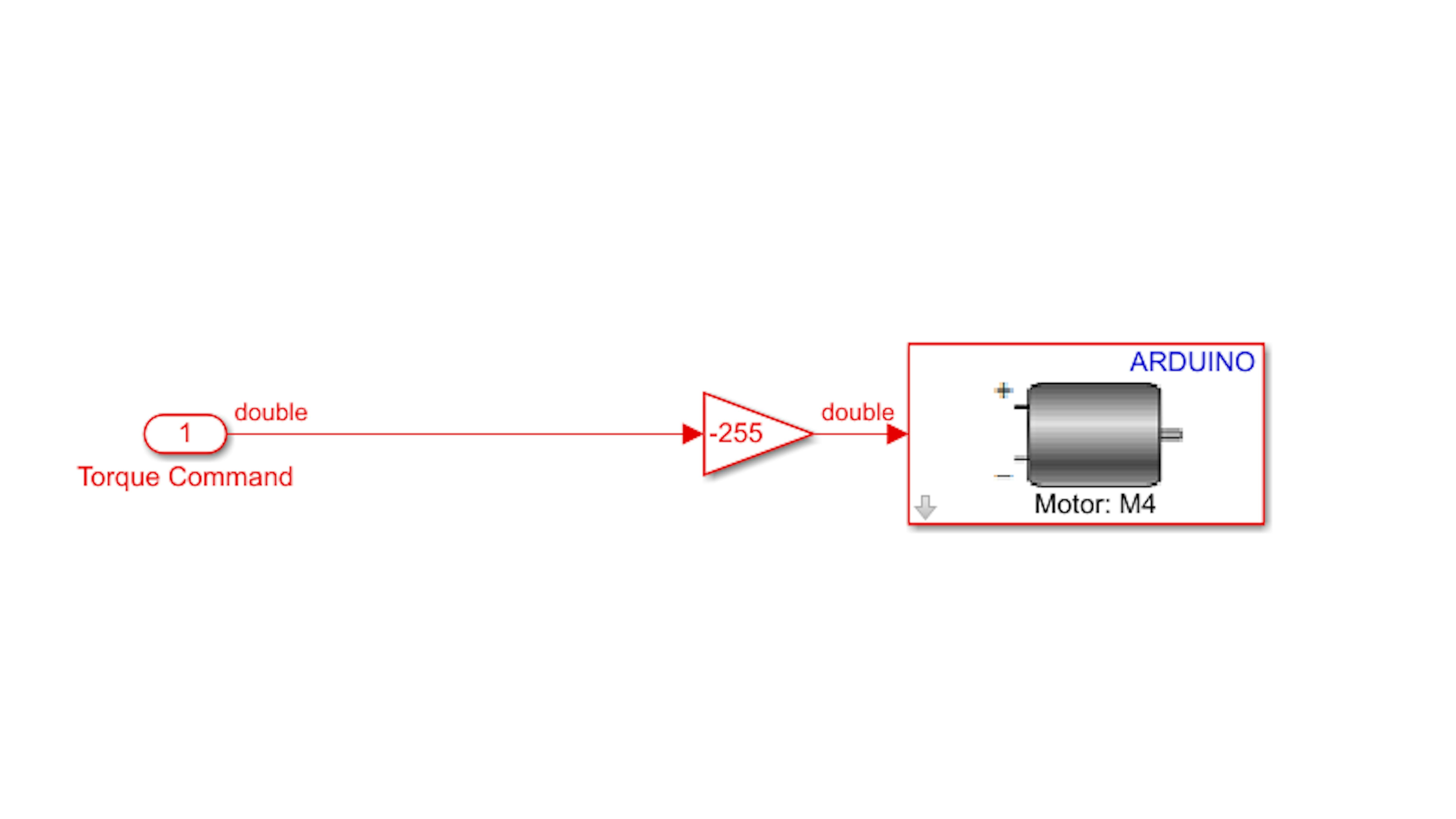
Reconnect the USB cable to PC and motorcycle and switch the power on the MKRMotorCarrier to ON (if it is switched OFF). Return to the top level of the model and run the model. Once the model is running, experiment with the manual switch, and change the Rear Wheel Torque Command values to set the speed to both positive and negative values (for safety purposes keep this below +/- 0.5):
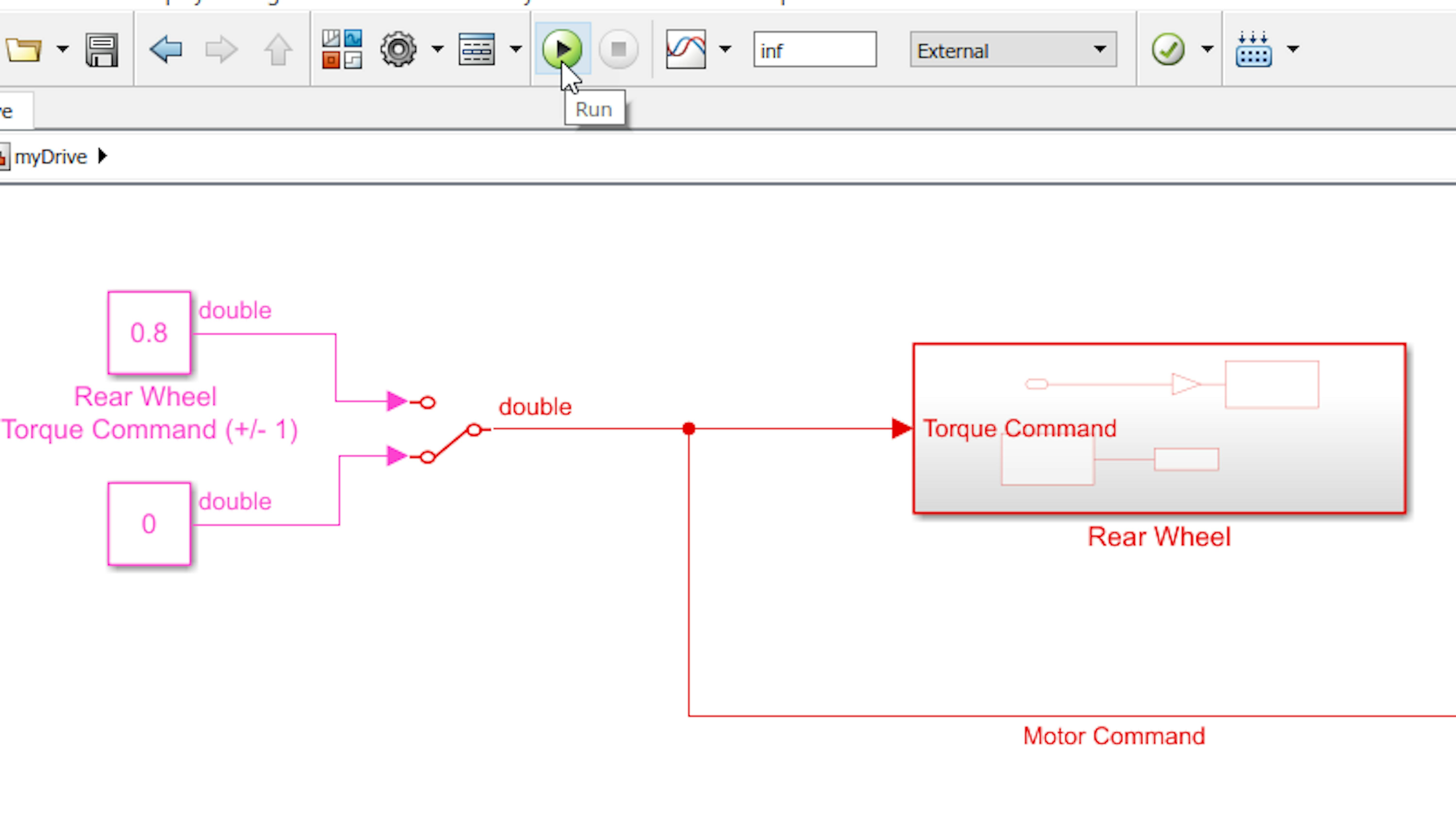
Examine the motion of the wheel with respect to the sign of the speed.
Does positive speed command result in forward propulsion of the motorcycle?
Disable the rear wheel and stop the model.
If your rear wheel did not give forward propulsive motion for a positive speed command, change the gain value inside the Rear Wheel subsystem from -255 to +255:

Note: the previous image is only meant to represent a case where you had to change the spinning direction of the motor.
Next, let’s try operating the rear wheel via Wi-Fi. In myDrive.slx, go to Configuration Parameters and navigate to the Hardware Implementation pane. Expand Target hardware resources and click WiFi properties. Enter your network credentials and click on Apply:

Next, click External mode and set Communication interface to WiFi:

Click OK.
Run the model. When the model begins to run, disconnect the USB cable from the front of the motorcycle (behind the front wheel). Try enabling the rear wheel and changing the speed value remotely.
Now, let’s try driving! First, disable the rear wheel motor using the manual switch. Then, restore the kickstand to its original diagonal position:

Note: Hold your motorcycle by the sides as there is no inertia wheel spinning in this model.
Place the motorcycle on the floor with plenty of room along the line of motion in both directions. Set the speed low to start (around 0.2) and enable the rear wheel. Experiment with different torque command values and try to drive the motorcycle.
Stop the model.
MEASURING MOTORCYCLE SPEED
Later, you will want to know how fast the motorcycle is moving so that you can calculate the ideal lean angle for a coordinated banked turn. To measure the longitudinal velocity of the motorcycle, you will use the rotary encoder device attached to the rear wheel motor:
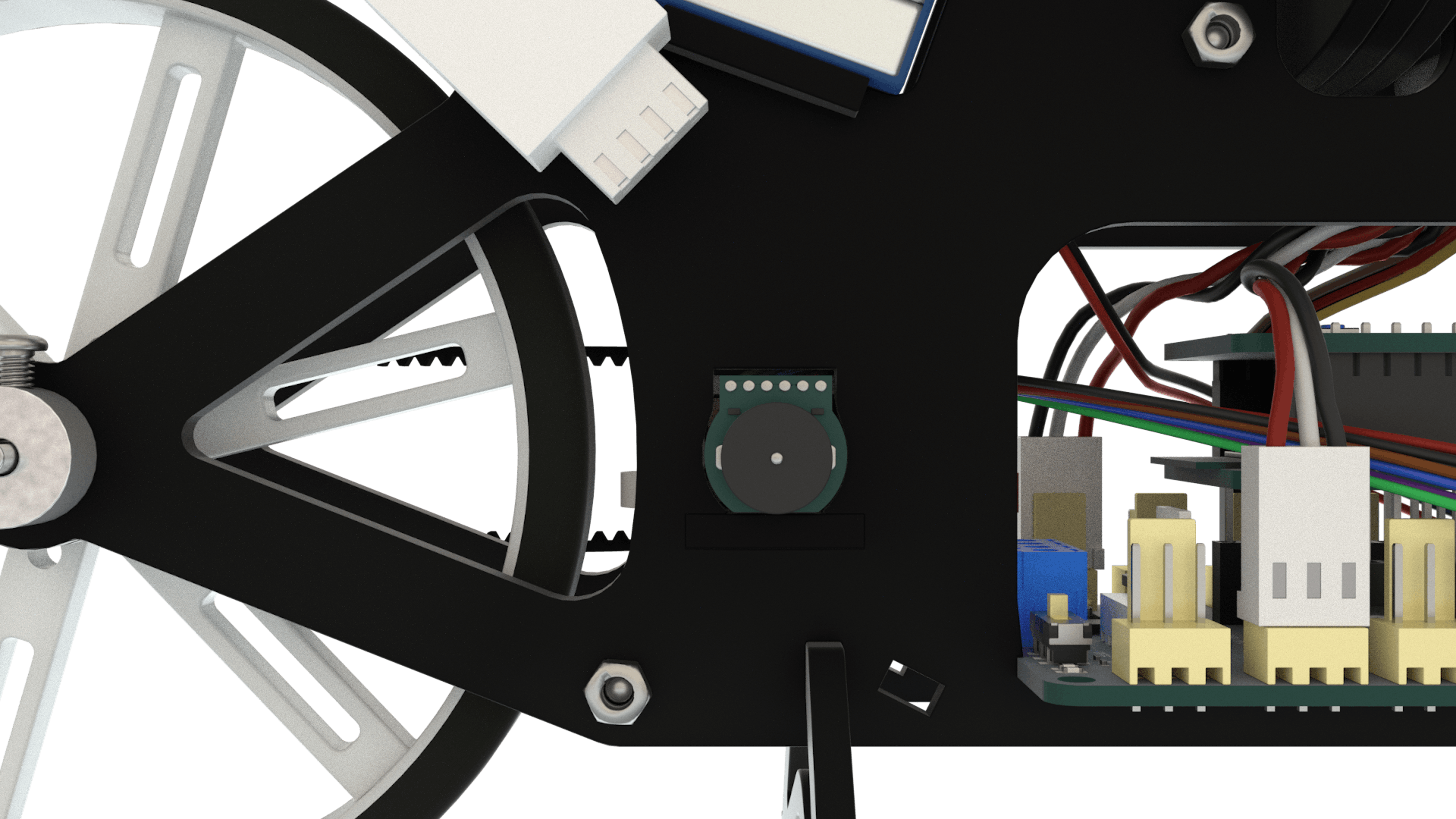
Recall from the introductory project in Chapter 2 that a magnetic rotary encoder detects the rotational motion of a motor shaft by measuring the field of a magnet that is rotating with the motor shaft. The motor carrier keeps track of the number of times the magnetic field has risen and fallen, as seen from two different rotational angles, and converts this information into an integer value. This integer value represents the angular displacement of the motor shaft since the counter was reset.
Return to the model myDrive.slx.
Note: If myDrive.slx is incomplete or unavailable, use drive2_wifi.slx instead. Remember to save this model as myDrive and configure the model to connect to your WiFi network.
Go inside the Rear Wheel subsystem (remember that the gain value may differ in your model because of the correction on the direction of movement):
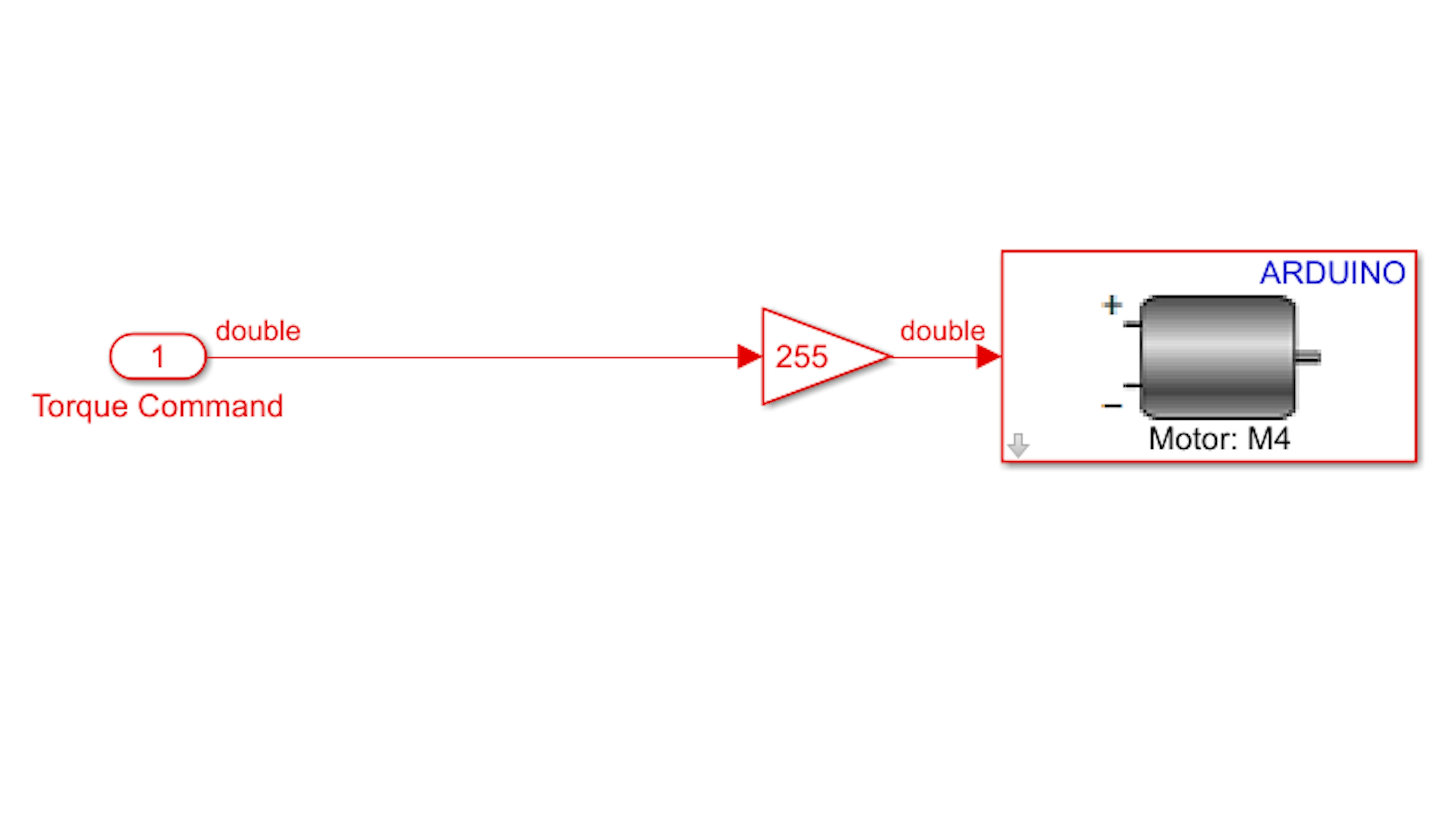
You will use the Encoder block to access the counter value.In the Simulink Library Browser, find the Encoder block in the Simulink Support for Arduino MKR Motor Carrier. Add the block to the Rear Wheel subsystem:

Check the wiring of your encoder:
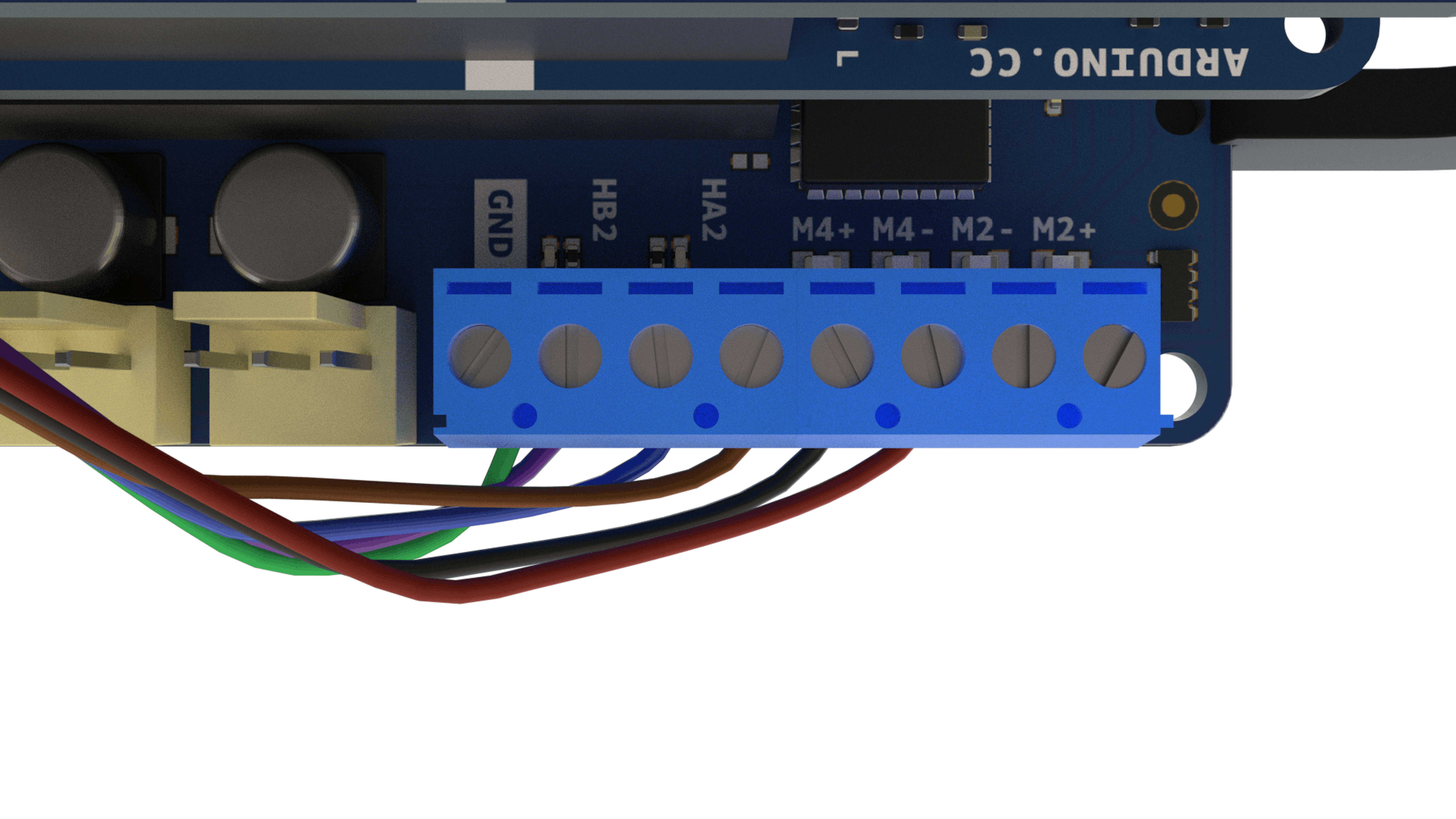
The motor carrier has 2 encoder ports, each consisting of 4 screw terminals. The middle 2 of the 4 screw terminals have labels HA1 and HB1, or HA2 and HB2. In the first case, you will read from Encoder 1, and in the second case, you will read from Encoder 2. Go into the Encoder block and set Encoder accordingly and change the Sample Time value to 0.01 as shown below:
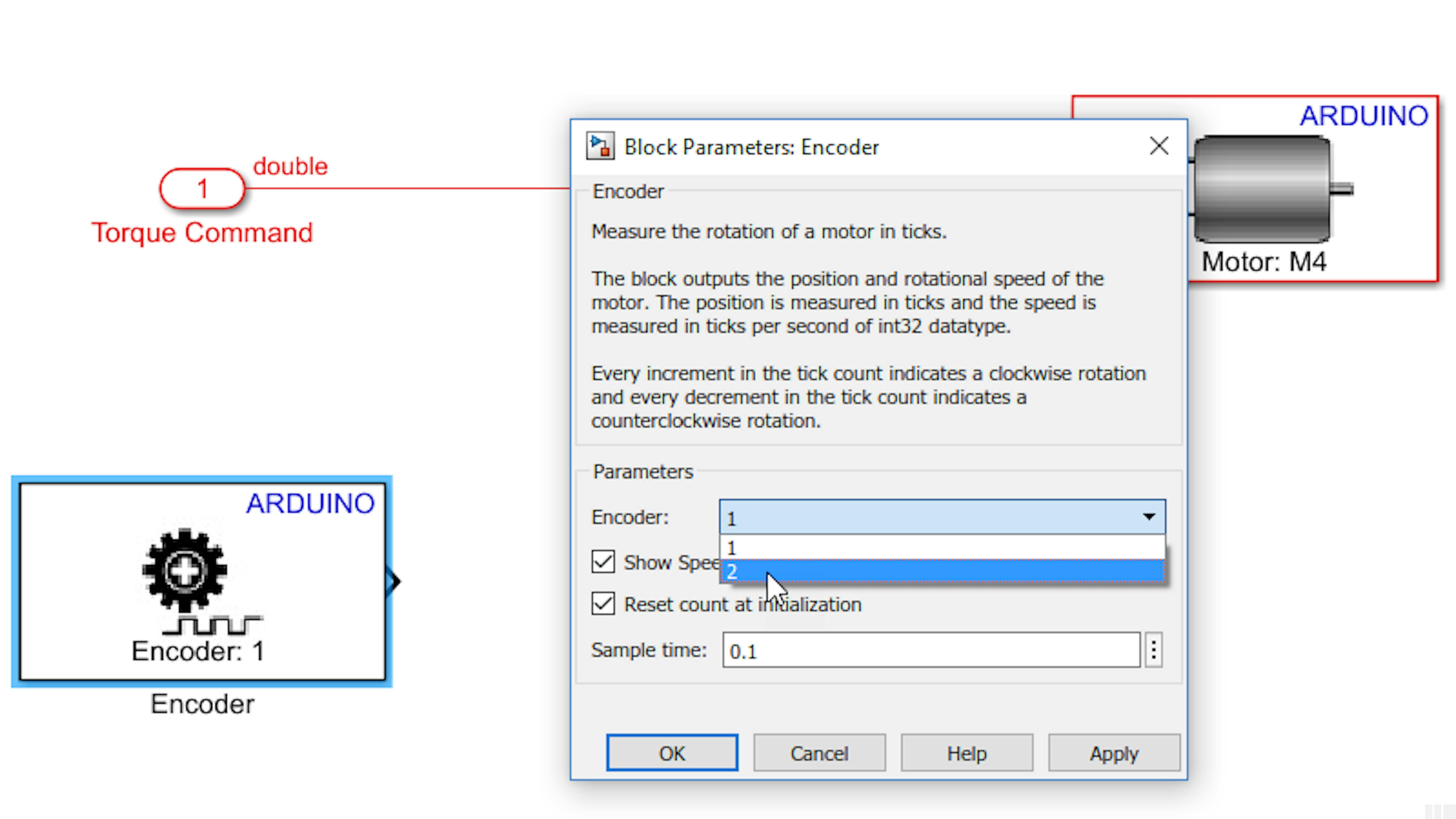
To test the encoder, add a Display block from Simulink → Sinks and connect it to the Encoder block’s outport:
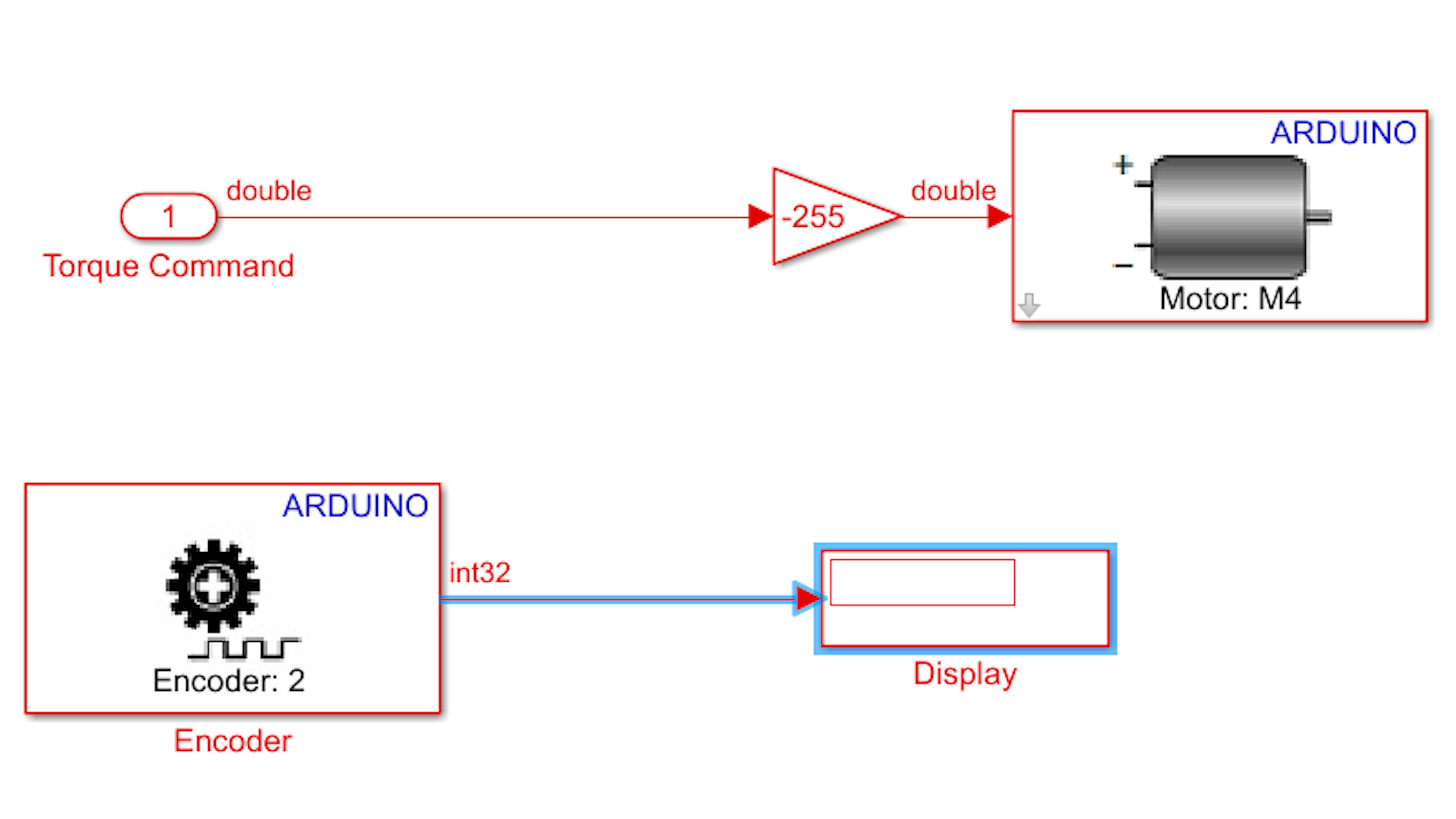
Make sure the rear wheel motor is disabled and run the model while you are still inside the Rear Wheel subsystem. Examine the display block:
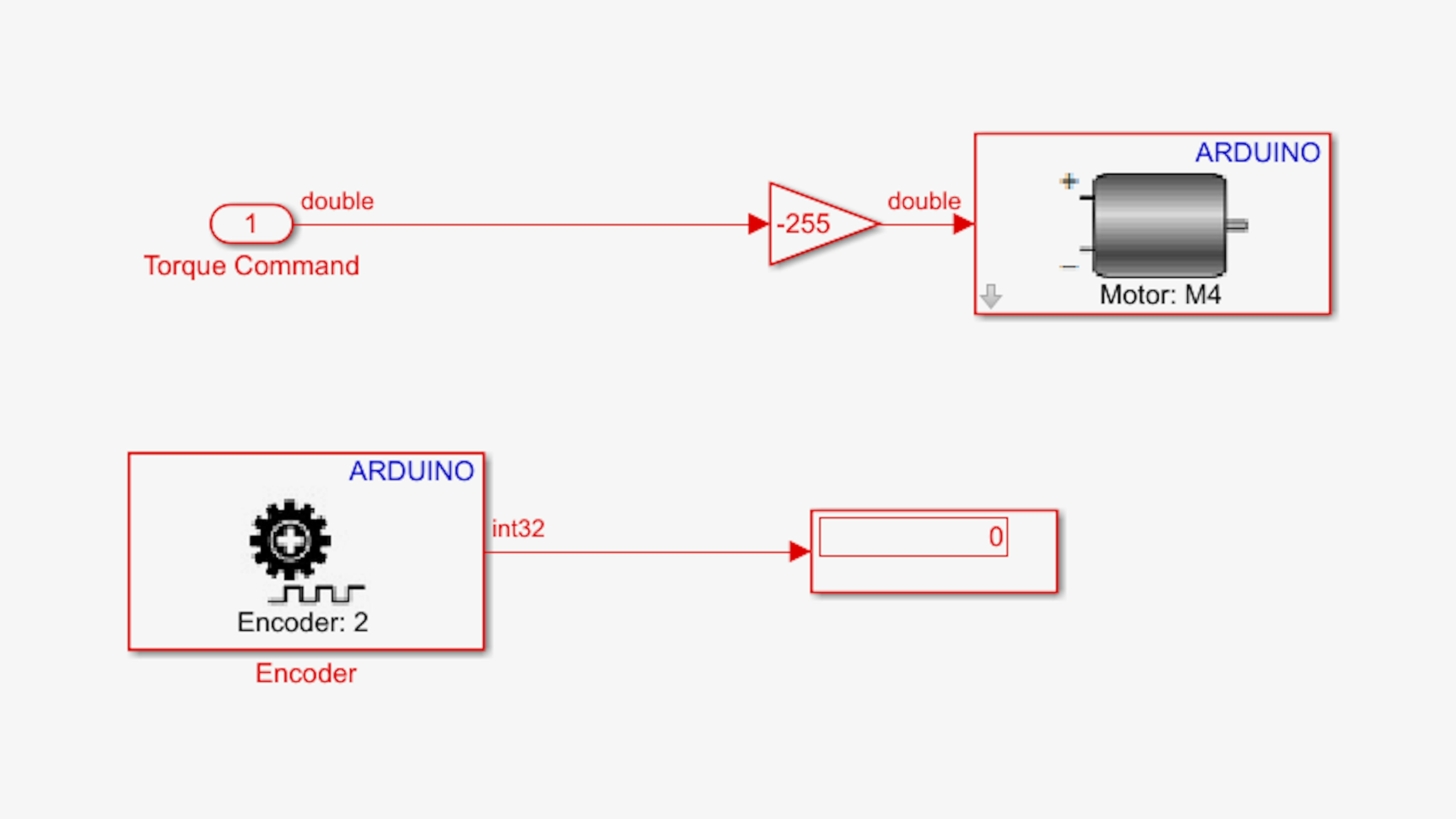
Now, manually rotate the magnetic encoder disk and you will see that the numbers on the display change:
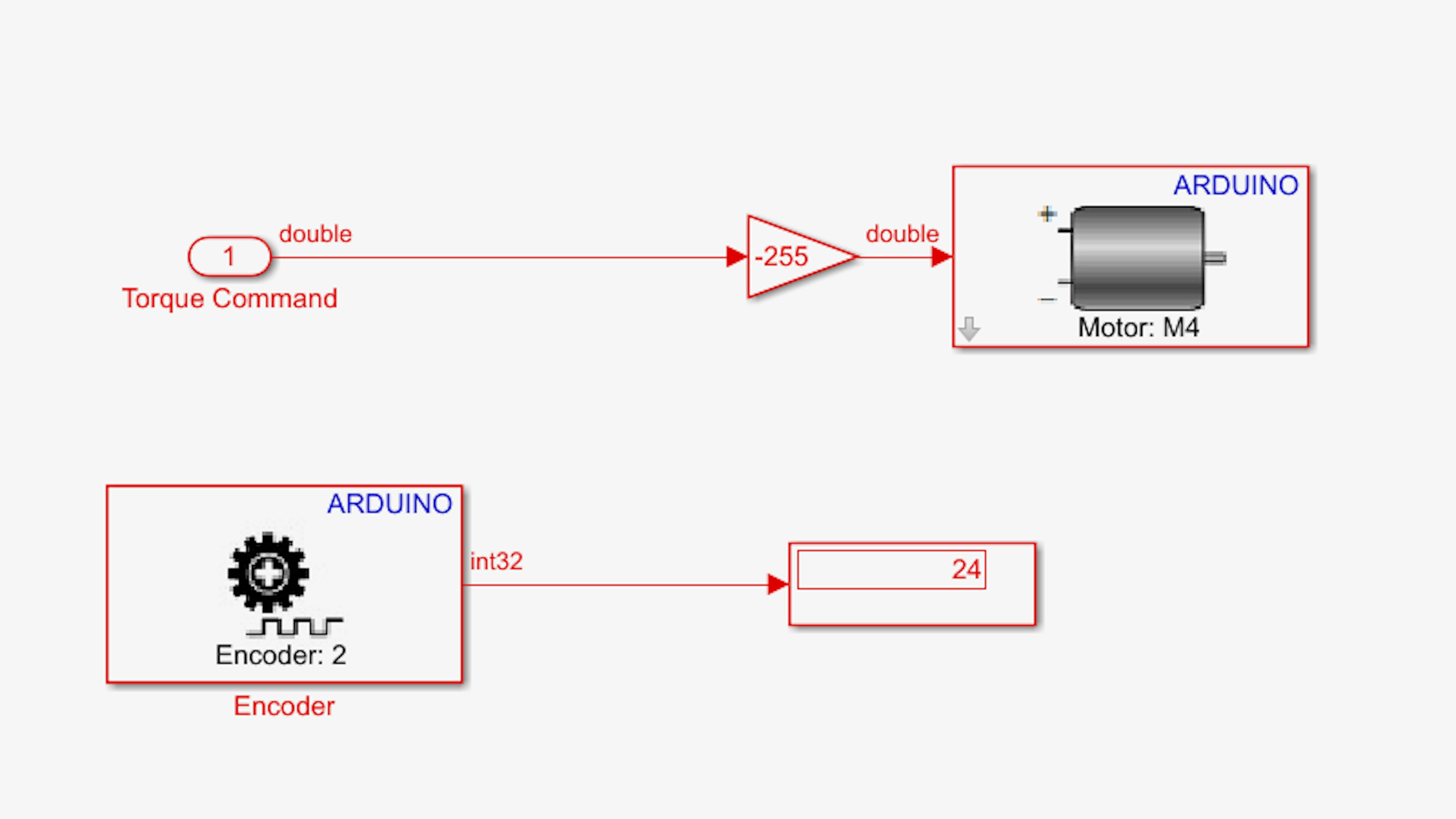
Take note of the sign of the encoder count. Stop the model.
This encoder has 12 counts per revolution of the motor shaft. The DC gear motor attached to the rear wheel spins the output shaft at 1/100 the rate of the motor shaft. This means that for each forward revolution of the rear wheel, we expect to see the encoder count increase by 12 x 100, or 1200 counts.
Now, let’s use the same technique from Chapter 2 to get the encoder speed. Delete the display block and add Unit Delay (Simulink → Discrete) and Sum (Simulink → Math Operations) block. Configure the Unit Delay and Sum block as shown below:
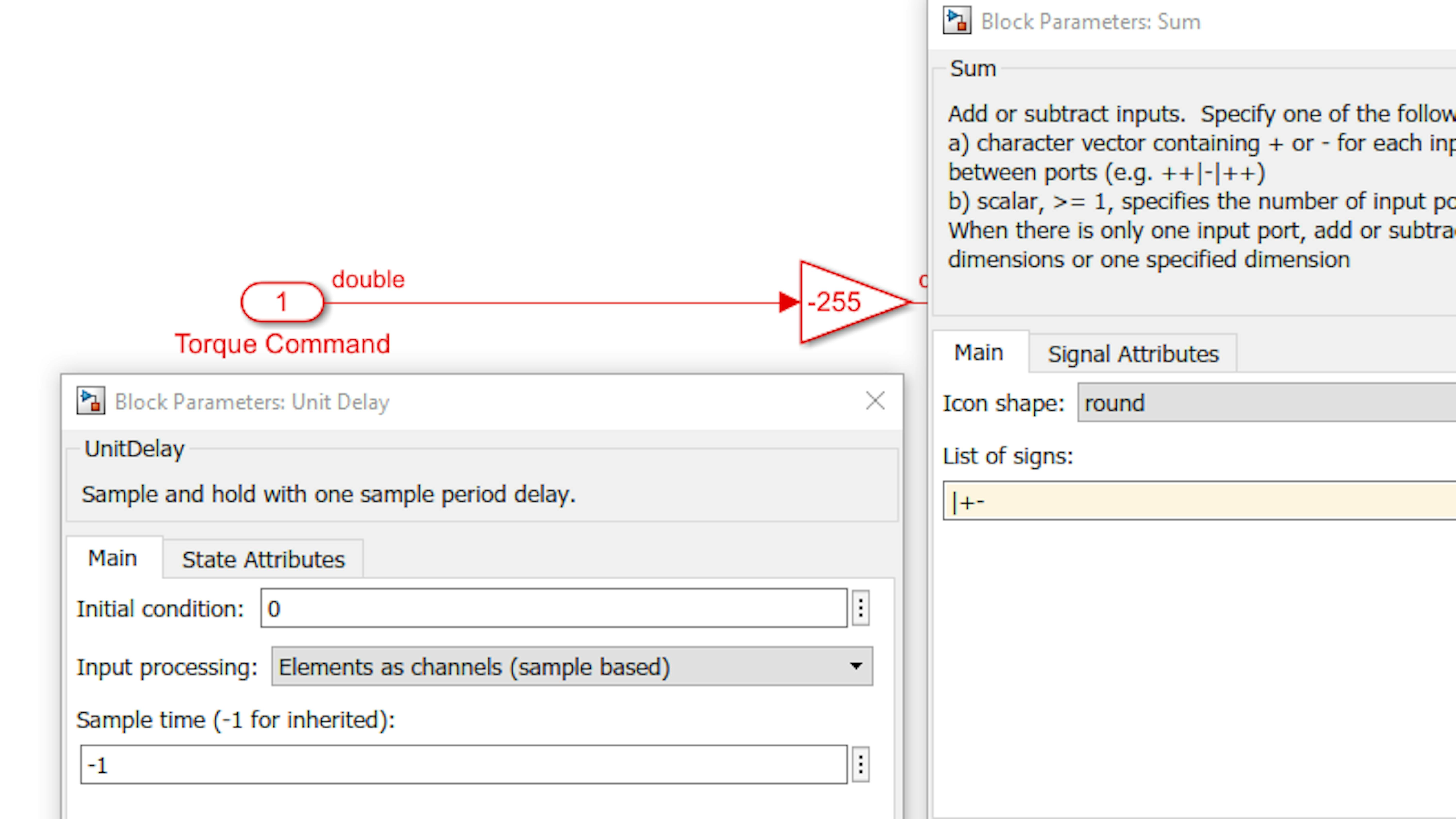
Next add a Gain (Simulink → MathOperations) block and change the gain value to “1/Ts”. Connect them all as shown below:

Add a Data type conversion (Simulink Signal Attributes) block in between the Sum and Gain block and change the output data type to “double”. The subsystem should look similar to this:
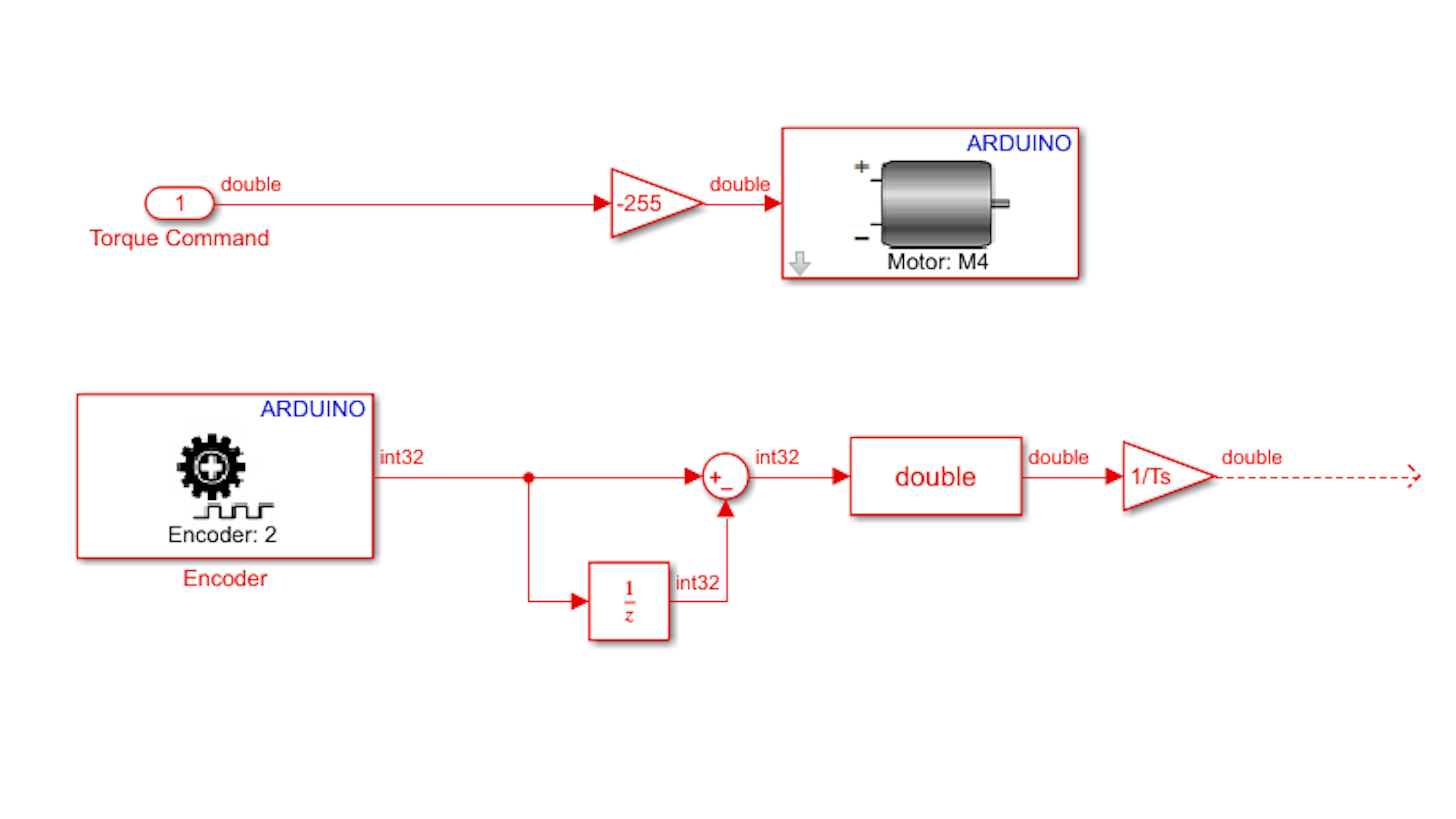
We want to express the speed in meters per second (m/s). This technique gives us speed in counts per second. We know there are 1200 counts per revolution of the rear wheel, and the circumference of the rear wheel is 2πr = 2π(45 mm) = 2π$$(0.045 m) = 0.2827 m. This means that to get the motorcycle speed in m/s, you need to multiply the speed in counts/s by 0.2827 m/1200 counts. Edit the Gain value of “1/Ts” to “(1/Ts)*(0.2827/1200)”.
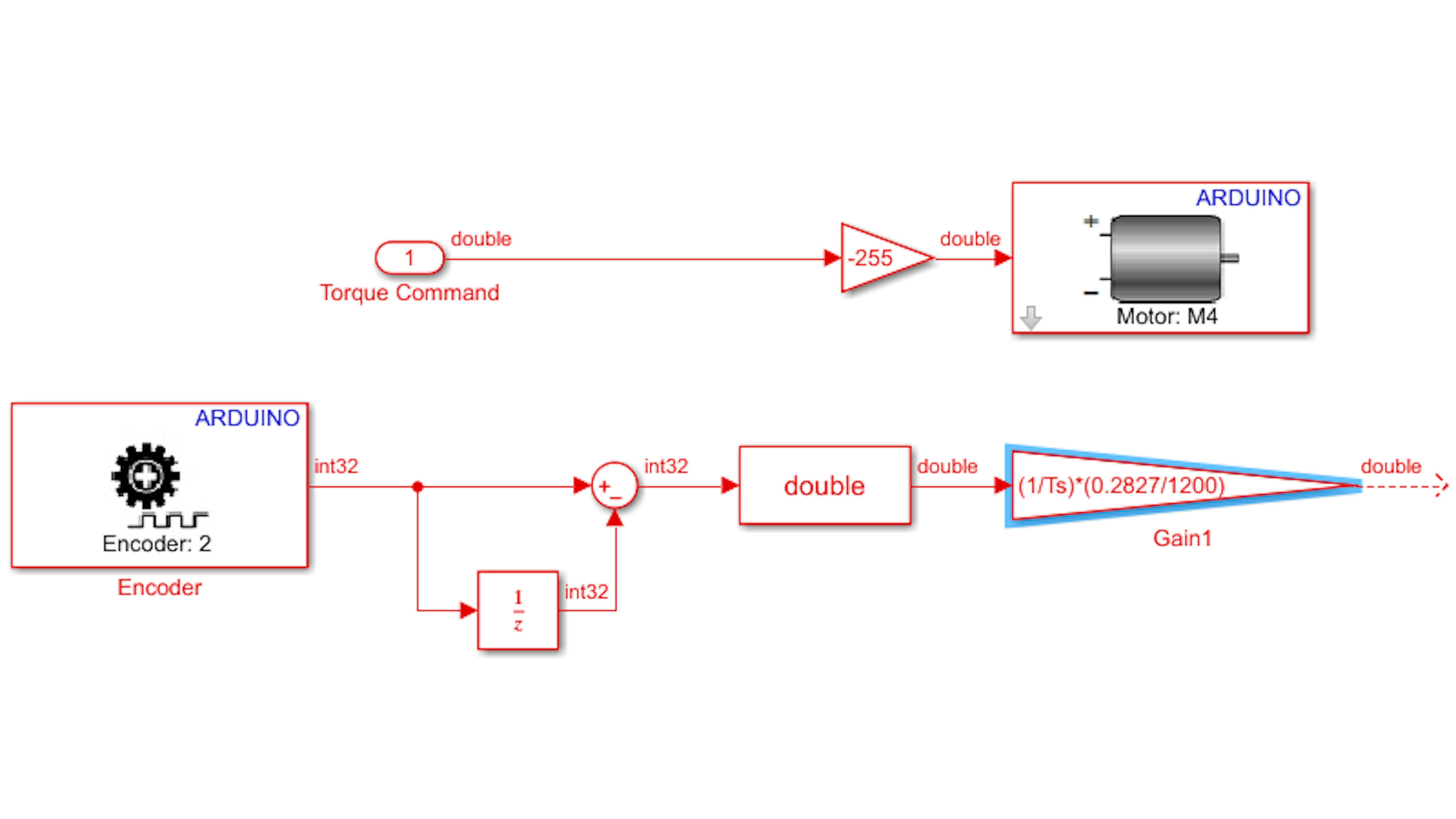
Note: If your encoder count gave a negative value when you turned the magnetic disk clockwise, use a gain of -0.2827/1200 instead.
Add an Out1 block from Simulink → Sinks to this subsystem and connect the encoder speed signal to this block. Name the output Rear Wheel Speed.
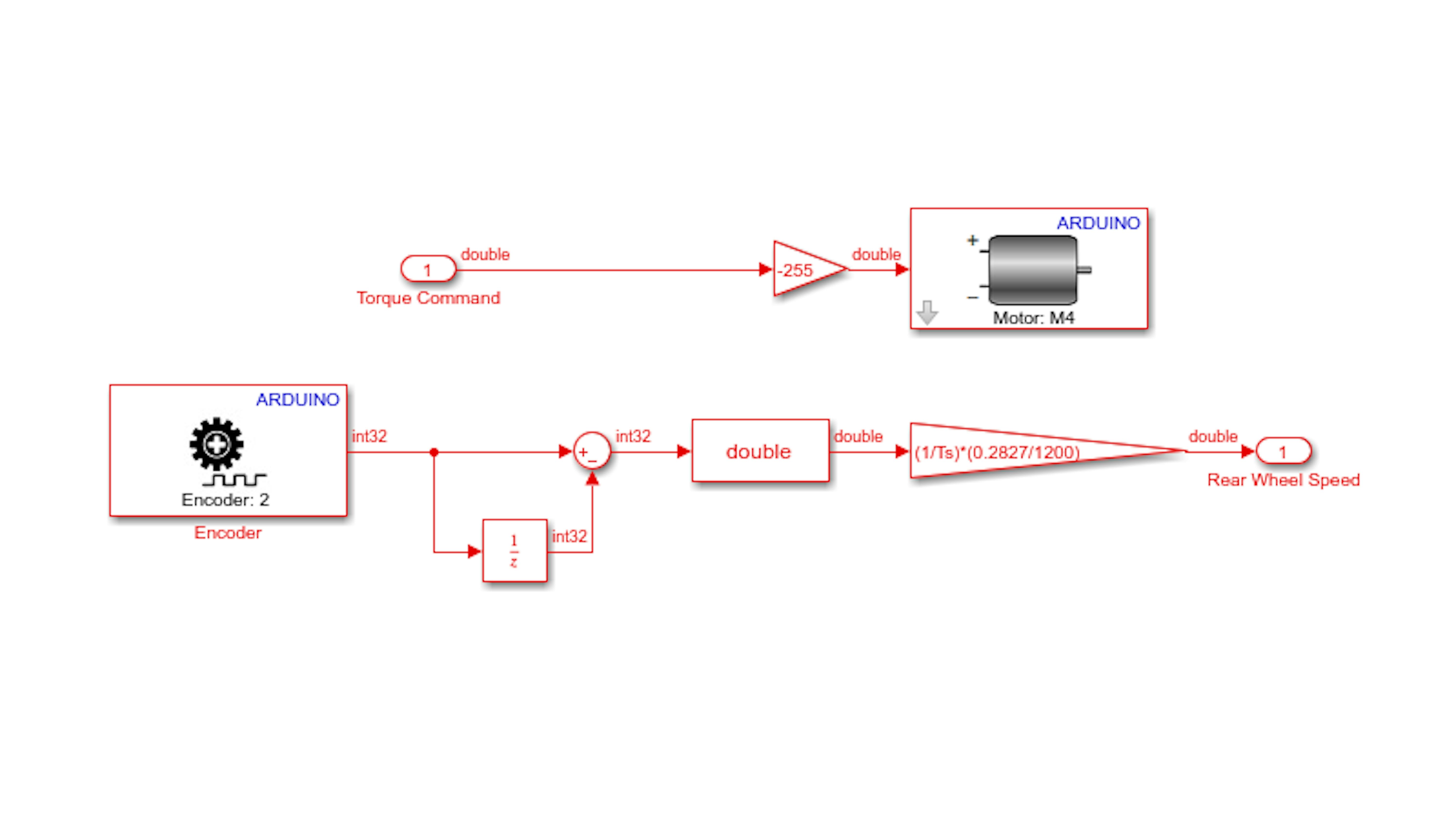
Go out to the top level of the model and feed the new subsystem output into the remaining Scope port. Label the signal "Rear Wheel Speed":

Before running the model, place the kickstand in the vertical position so that the rear wheel is off the ground surface:

Run the model and adjust the rear wheel speed by changing the torque command. Examine the Scope window and note the relationship between the torque command and the wheel speed:
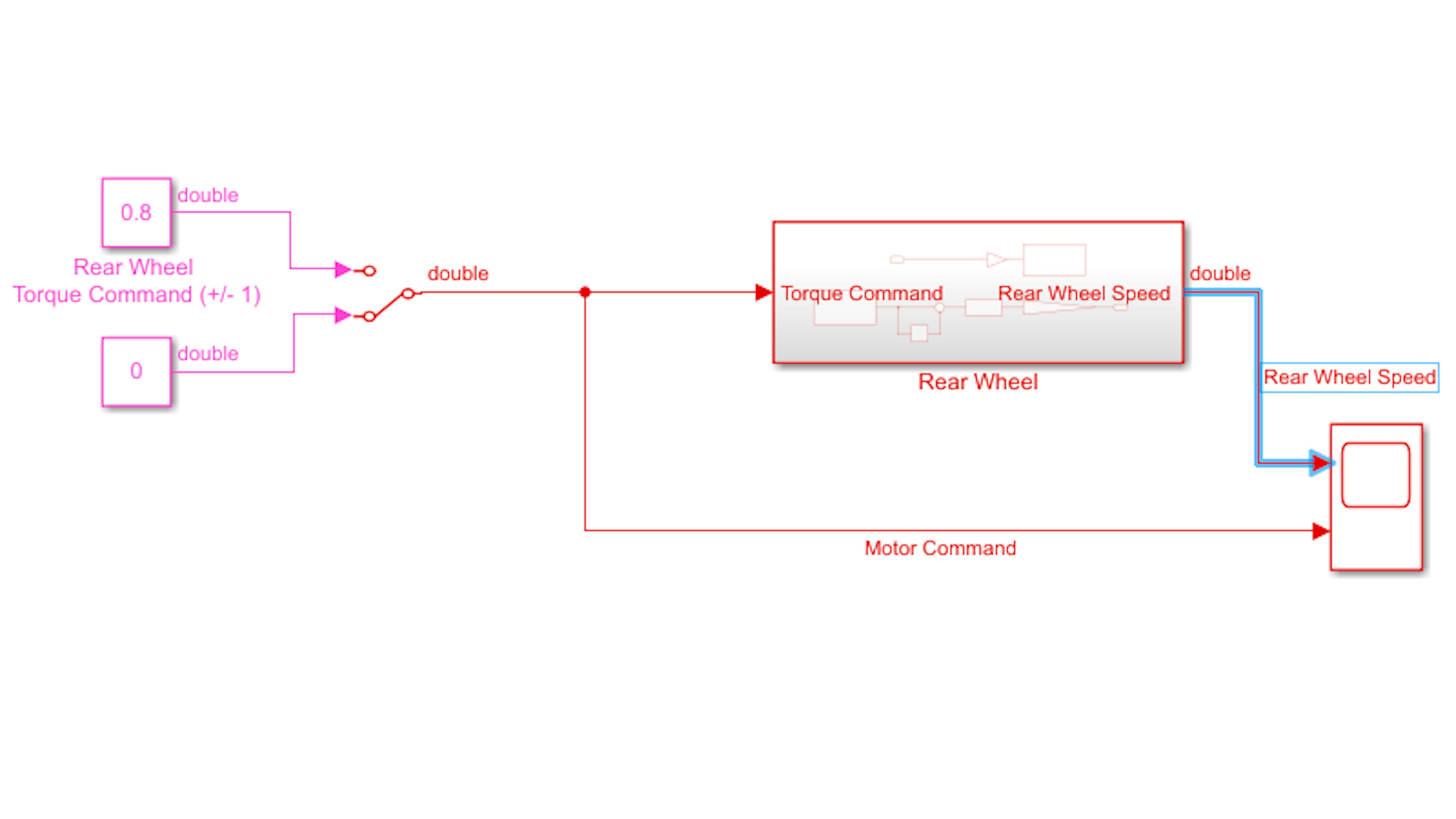
Note: The commanded torque values and the rear wheel speed are in different units. It is purely coincidental that they are similar magnitude in this image.
Disable the rear wheel (but keep the model running) and set the kickstand to its diagonal position. Disconnect the USB cable from the motorcycle and try driving the motorcycle on the floor. What happens to the motorcycle speed when the rear wheel is actually pushing the motorcycle? You should observe the motorcycle speed decreases for a given motor command when the wheel is propelling the weight of the motorcycle.
BALANCING WHILE DRIVING IN A STRAIGHT LINE
Now let’s integrate the rear wheel into the system model, and attempt to balance the motorcycle with forward and backward motion. Copy all the blocks from myDrive.slx to myNewMoto.slx except for the Scope block and lay out the model approximately as shown:
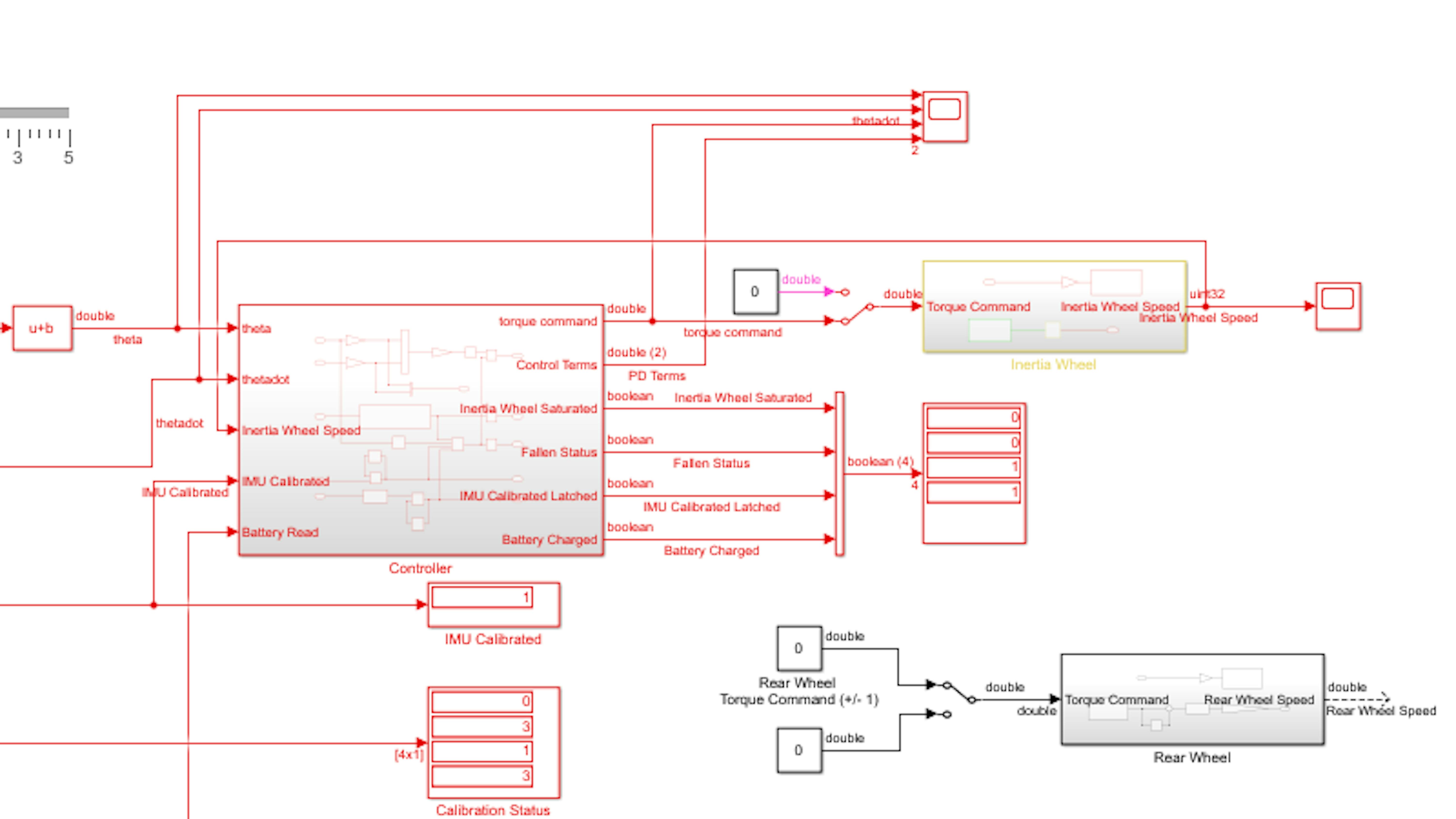
Now drag the rear wheel speed signal from the Rear Wheel subsystem outport to the Scope block, creating a second input to the Scope block:
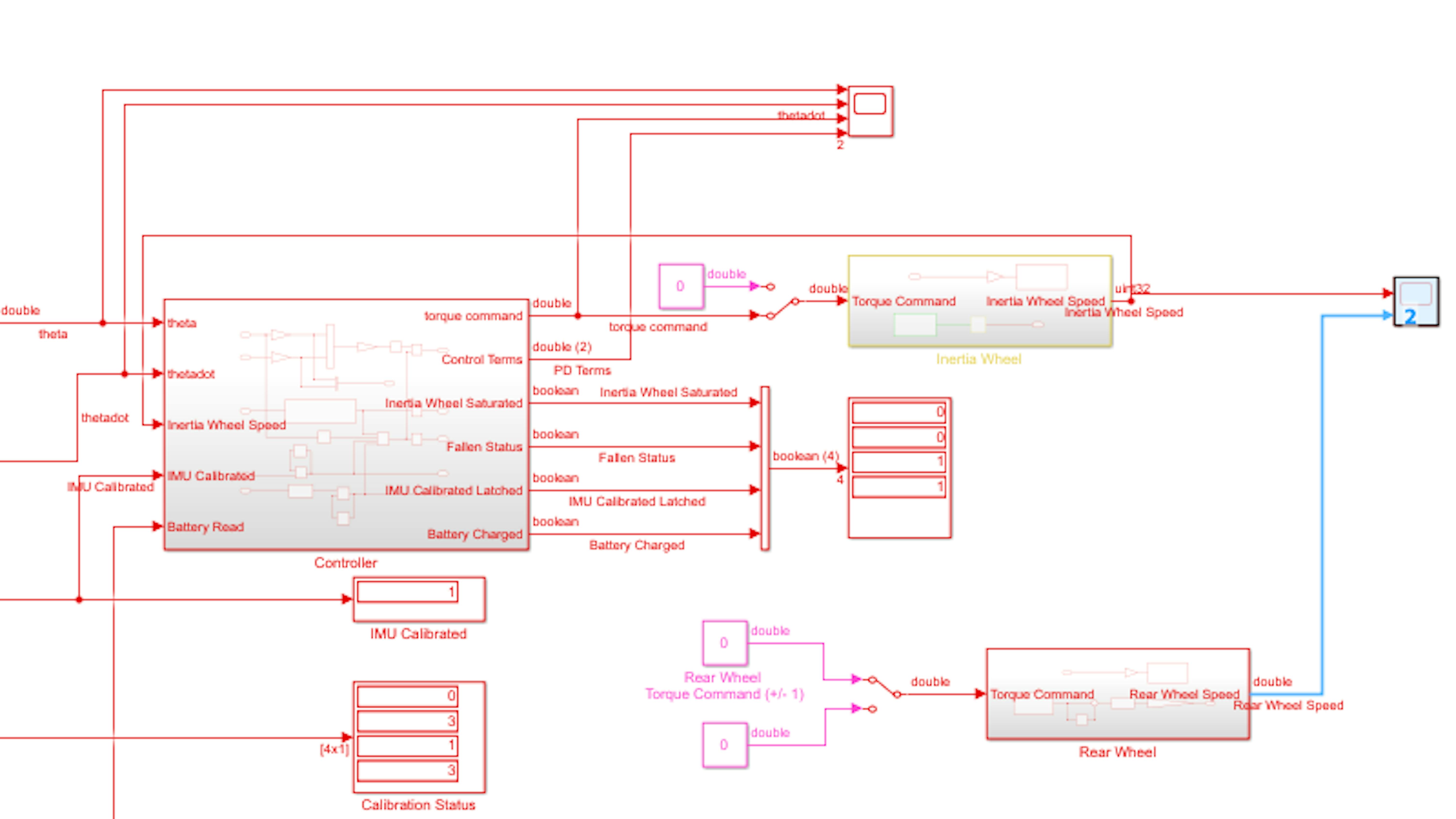
Ensure that the kickstand is not in the vertical position. Run the model and examine the Scope window. Make sure the IMU gets calibrated. Enable the inertia wheel if it is not already enabled and ensure that the motorcycle balances in place, using the techniques from the previous exercise.
Test the rear wheel while holding the motorcycle (so that it doesn’t drive away).
With the model still running, disable the rear wheel and set the torque command to 0.3. Next, disconnect the USB cable from the motorcycle and place it on the floor. Balance the motorcycle in place. Once you have the motorcycle balancing stably with low inertia wheel acceleration, enable the rear wheel using the manual switch. If the motorcycle remains upright, try changing the rear wheel torque command, stopping, and driving in reverse.
Balancing the motorcycle while in motion may take some trial and error. Here are some troubleshooting tips:
- Be sure to prevent jolts in the rear wheel motion by modifying the value in small increments.
- Ensure that the timing belt connecting the DC motor shaft to the rear wheel axle is catching the teeth on the guide wheels.
- Ensure that the guide wheels are fastened securely to their respective axles.
- Ensure that the front wheel is pointing directly forward (motorcycle is not steering left or right). You can manually rotate the steering column so that it is aligned with the motorcycle body.
How does smooth longitudinal motion affect the stability of the balance controller?
LEARN BY DOING
In this chapter, you tested and integrated two new hardware devices – the rear wheel gear motor and the rear wheel rotary encoder. This enables you to move the motorcycle forward and backward with varying speed. You also configured the main system model to communicate with the MKR1000 via Wi-Fi so that you can run and monitor the balance control application without the USB cable connected to the motorcycle. You then learned how to balance the motorcycle while it is moving in a straight line.
In the current model, you are sending a PWM command to the rear wheel motor to exert some known amount of torque on the rear wheel to propel the motorcycle forward or backward. The resulting speed of the motorcycle depends on many factors, such as the weight of the motorcycle, the slope of the surface it is driving on, whether the motorcycle is balanced or leaning on its training wheels, and the remaining charge in the battery. In other words, setting the motor torque to a certain value does not result in the motorcycle moving at a precisely known speed. You can see this by observing the rear wheel speed in the Scope window.
As an extra challenge, try to find the relationship between the motorcycle’s forward speed and the applied rear wheel motor torque when the motorcycle is driving on flat smooth ground with a full battery and while balancing. Then, in the Simulink model, calculate the rear wheel torque command as a function of desired speed and allow the model’s user to set the speed directly in meters per second. Make sure that the torque command is not allowed to saturate or stay close to its limits for too long (so that you do not burn out the motor).
EXERCISE 5:
6.5 Balancing while steering
In this exercise, you will learn how to control the servo motor that steers the motorcycle left and right. Once you have the steer servo working, you will be able to drive the motorcycle along arbitrarily curved paths on the ground. You will then test whether your control algorithm can achieve balance while the motorcycle is turning. You will see that the turning action causes an extra torque component to be applied to the motorcycle about the wheel-ground axis, which then requires the inertia wheel to compensate. In this exercise, you will balance the motorcycle only on turns with a large turn radius. If you continue to the final challenge following this exercise, you will modify the controller to compensate for the extra torque by leaning into the turn, or banking.
In this exercise, you will learn the following:
- Understand the capabilities and relevant specifications for the steer servo motor.
- Test and integrate the steer servo motor into the motorcycle application so that the motorcycle can move along arbitrary paths.
- Balance the motorcycle while driving with a large turn radius (small steer angle).
CONTROLLING STEER SERVO
The motorcycle is equipped with a servo motor in the steer column. Take a moment to look at the hardware specifications of the GS-9025MG servo motor. This servo motor can rotate its lever arm to any angle between 0 and 180 degrees. If you manually rotate the steer column, you will see that the range of motion does not cover 180 degrees, but rather closer to 60 degrees.
We’ll start by testing the servo motor in isolation. Open the model myDrive.slx:
Note: If myDrive.slx is incomplete or unavailable, use the model drive3_encoder.slx and save it as myDrive.slx.
Recall that this model is configured to perform External mode communications via your Wi-Fi network. Make sure your computer is connected to the Wi-Fi network that you used in the previous section. If connecting to a new Wi-Fi network, make sure you change the Wi-Fi credentials in Configuration Parameters like you did in Section 6.4 “Controlling and Monitoring Motorcycle via Wi-Fi”.
In the Simulink Library Browser, navigate to Simulink Support for Arduino MKR Motor Carrier and locate the Servo Write block. Add it to myDrive.slx:
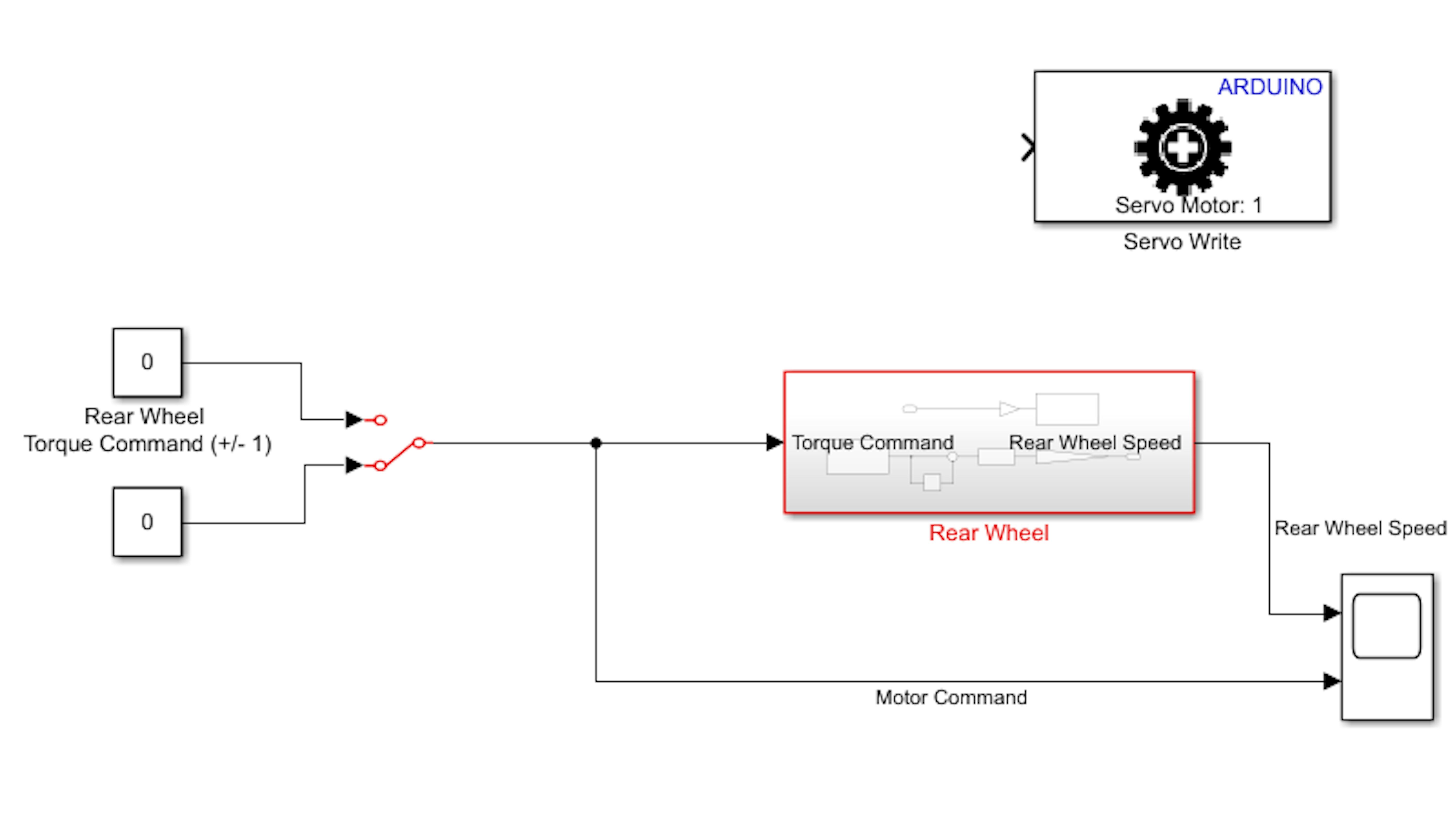
Examine your motor carrier. The servo motor should be plugged into SERVO3 which is one of 4 servo ports on the motor carrier labeled SERVON where N is between 1 and 4:
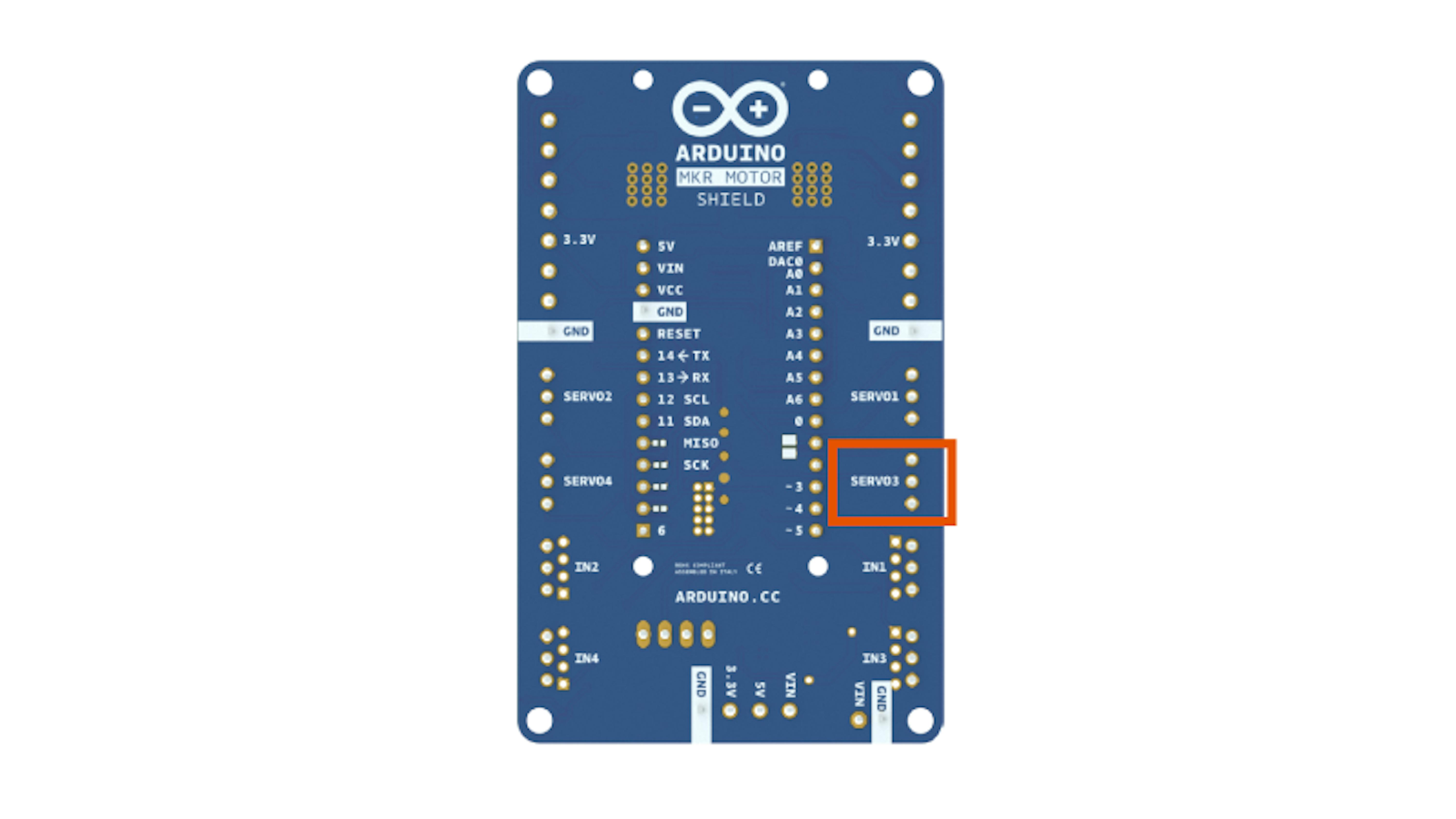
Open the Servo Write block dialog and set Motor port to 3 and click OK:
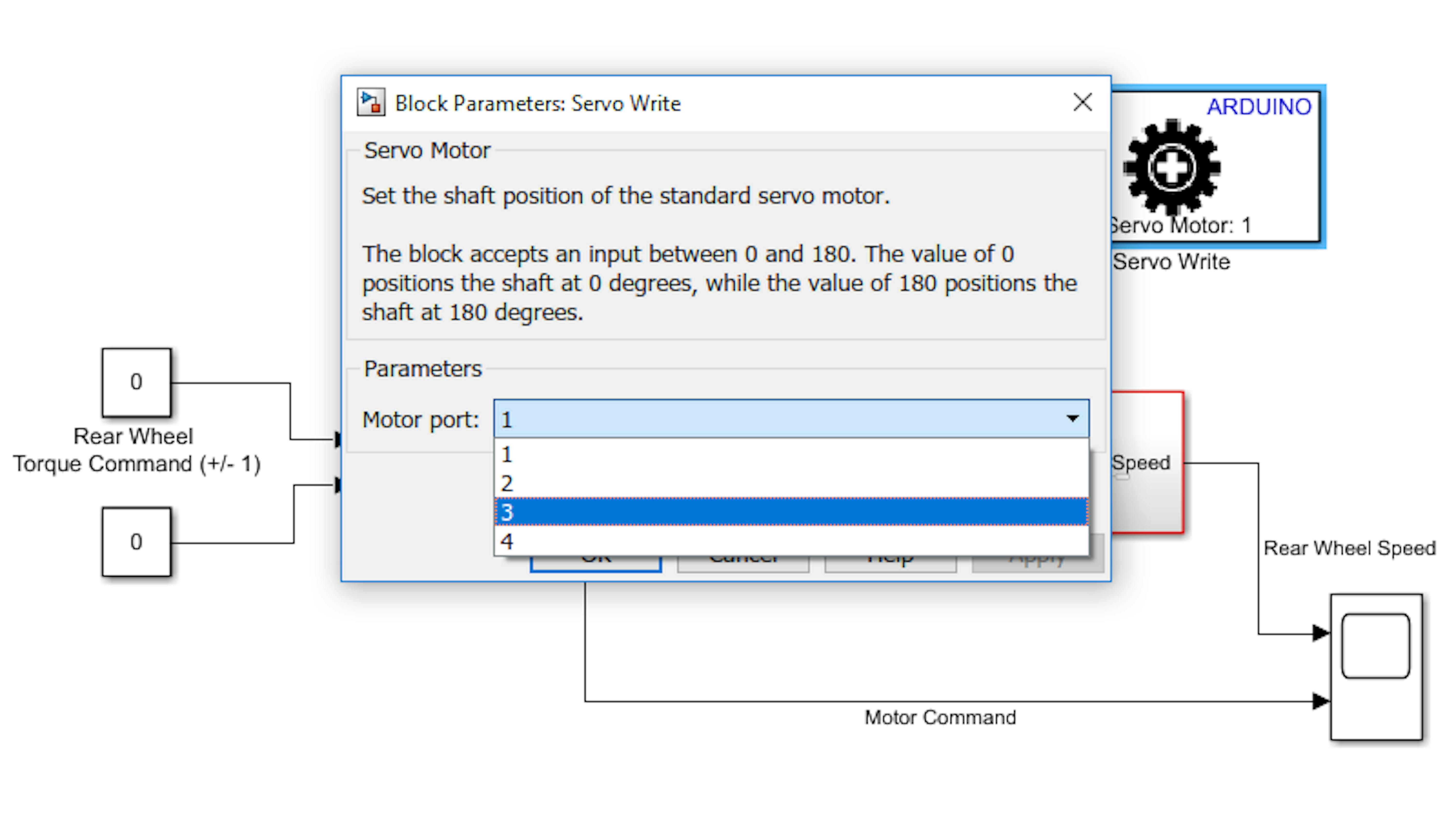
The servo motor has 3 wires. The brown (sometimes black) wire is connected to electrical ground. The red wire connects to the reference voltage, which, in this case, is 5 V. The yellow (sometimes orange) wire is the signal wire and transmits the desired servo angle as a PWM signal. The wires should be oriented such that the ground wire (brown or black) is closest to the rear of the motorcycle and the signal wire (yellow or orange) is closest to the front of the motorcycle. If this is not the case, unplug the servo motor from the motor carrier and reverse the orientation:
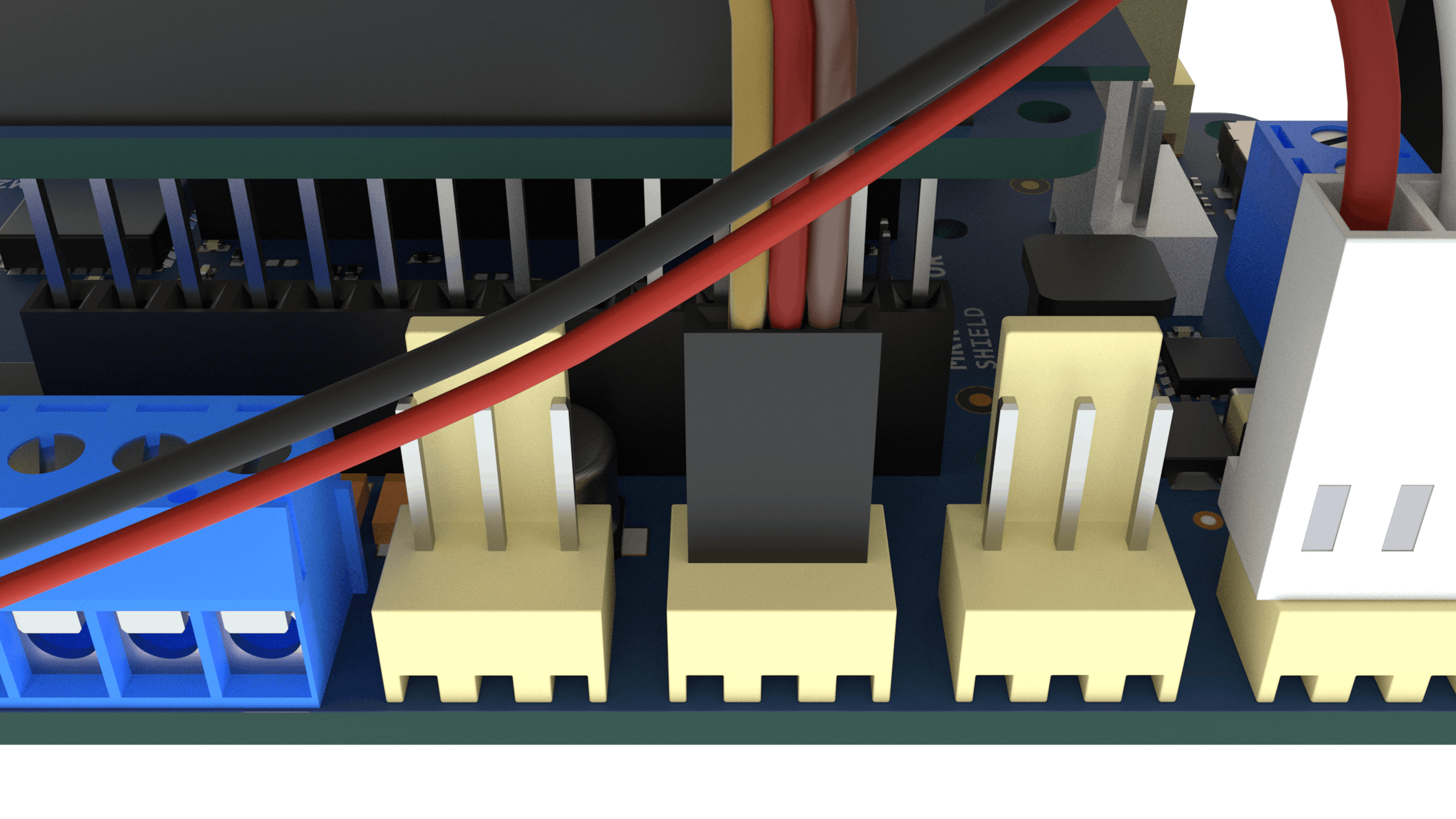
Note: If you followed the assembly instructions video accurately, you will not have to change the servo motor wiring.
Now, let’s test the steer servo. Add a Constant block from Simulink → Sources and set the value to 90. Connect as shown:
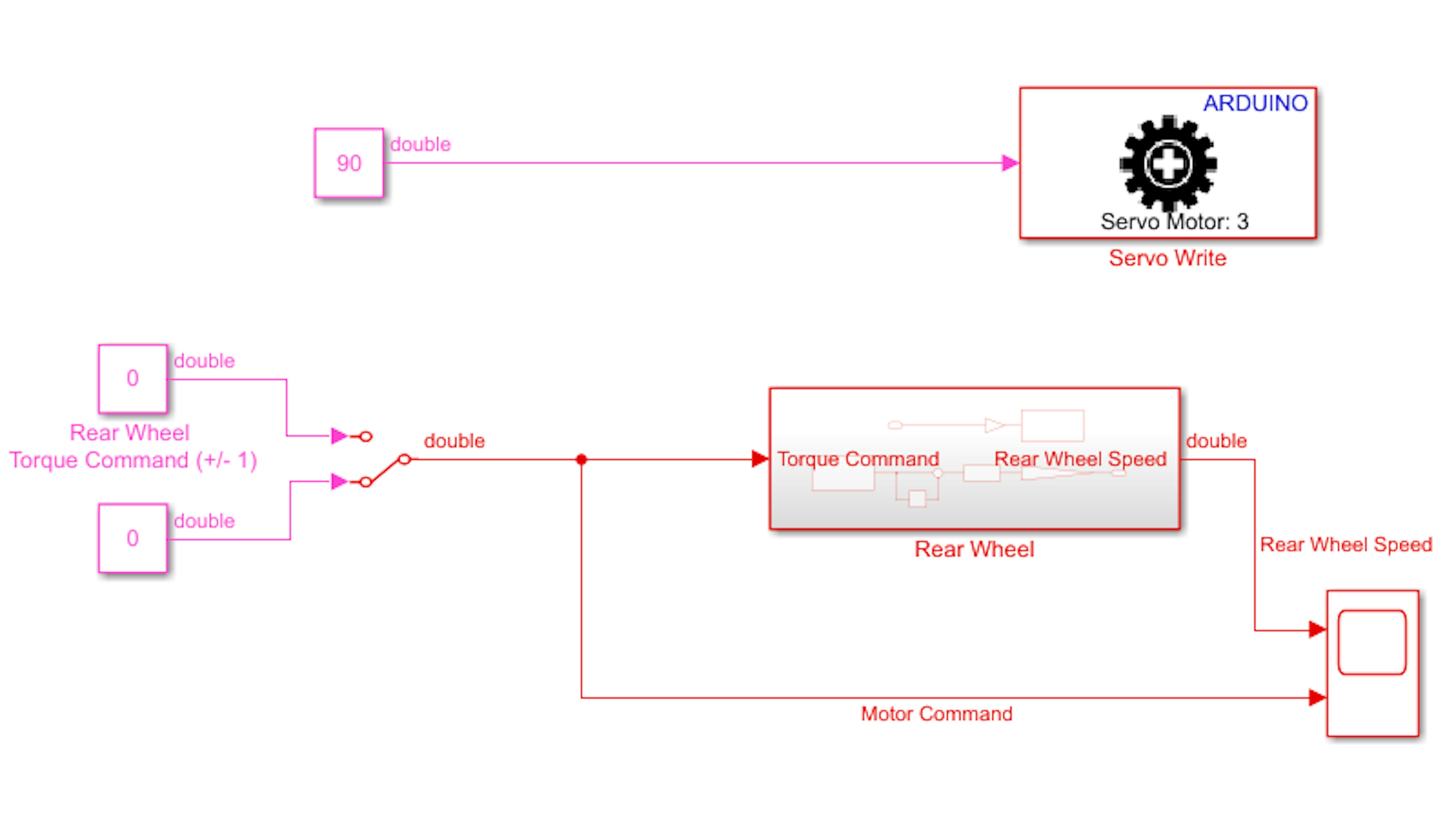
The Servo Write block takes input values between 0 and 180. The motorcycle is constructed such that the “straight” angle is approximately 90 degrees, but this needs to be checked and calibrated.
Run the model. Try changing the value in the Constant block while the model runs in External mode. Click Apply in the Constant block dialog window to implement new servo inputs:
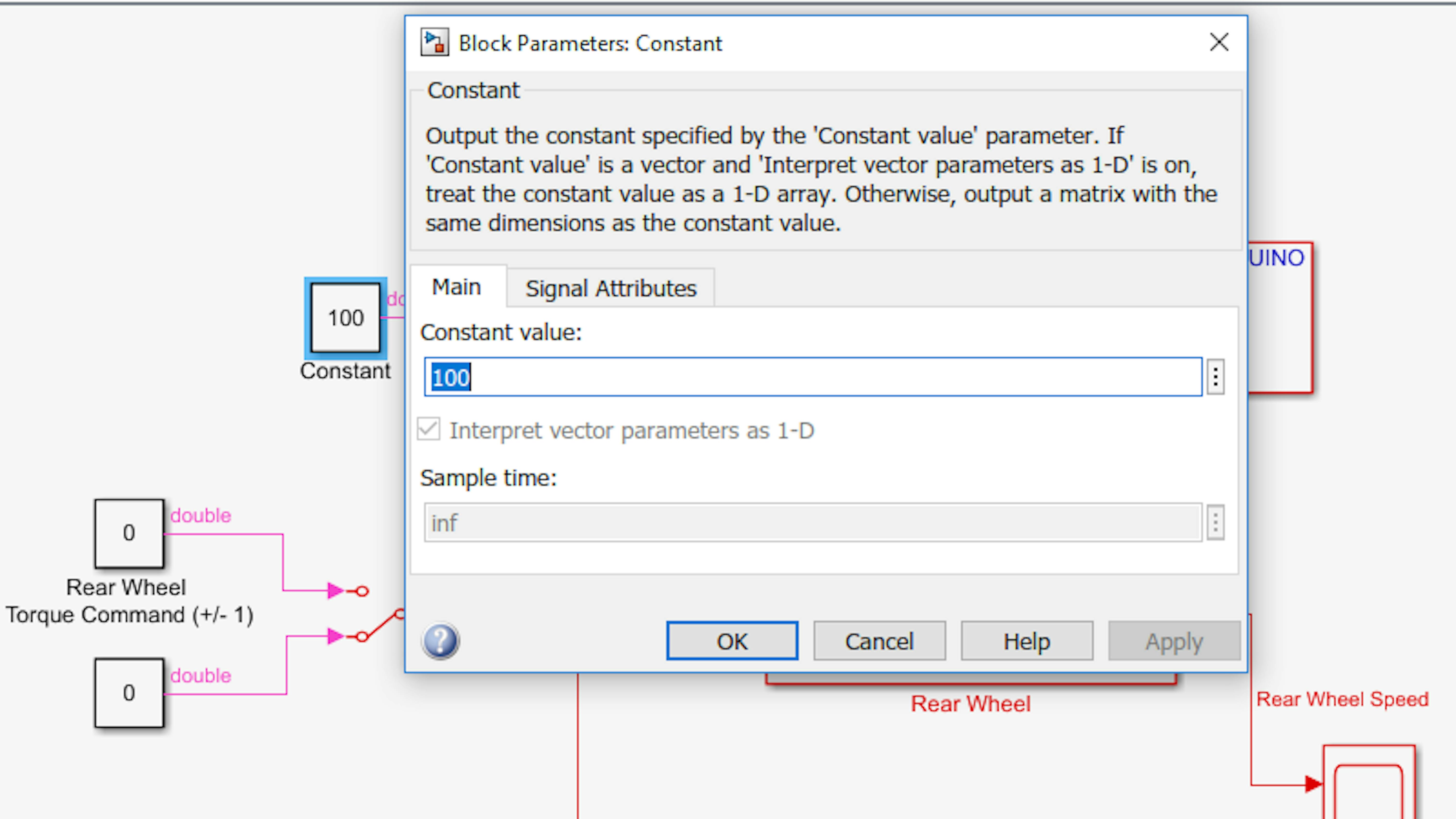
Note that there are physical limits to how much the servo can rotate due to the mechanical construction of the motorcycle. Let’s try to figure those out empirically. Using the Constant block dialog window, find the angle at which the steer column hits a hard stop on the left (the value at which the servo can no longer turn farther to the left). In our tests this was 120 degrees and this is the maximum value that you should ever command to this servo motor. You can command higher values, but the servo will attempt to drive through the motorcycle frame, which could stress and damage the servo and frame.
Now, find the angle at which the steer column hits the hard stop to the right. In our tests this was 60 degrees and this is the minimum value that you should command to the servo.
Stop the model.
Let’s saturate the steer command to prevent commanding steer angles that will damage the motorcycle hardware. Add a Saturation block from Simulink → Discontinuities and place it in front of the Servo Write block. Set the saturation limits according to the minimum and maximum angles you measured previously (in our case 60 and 120, respectively):
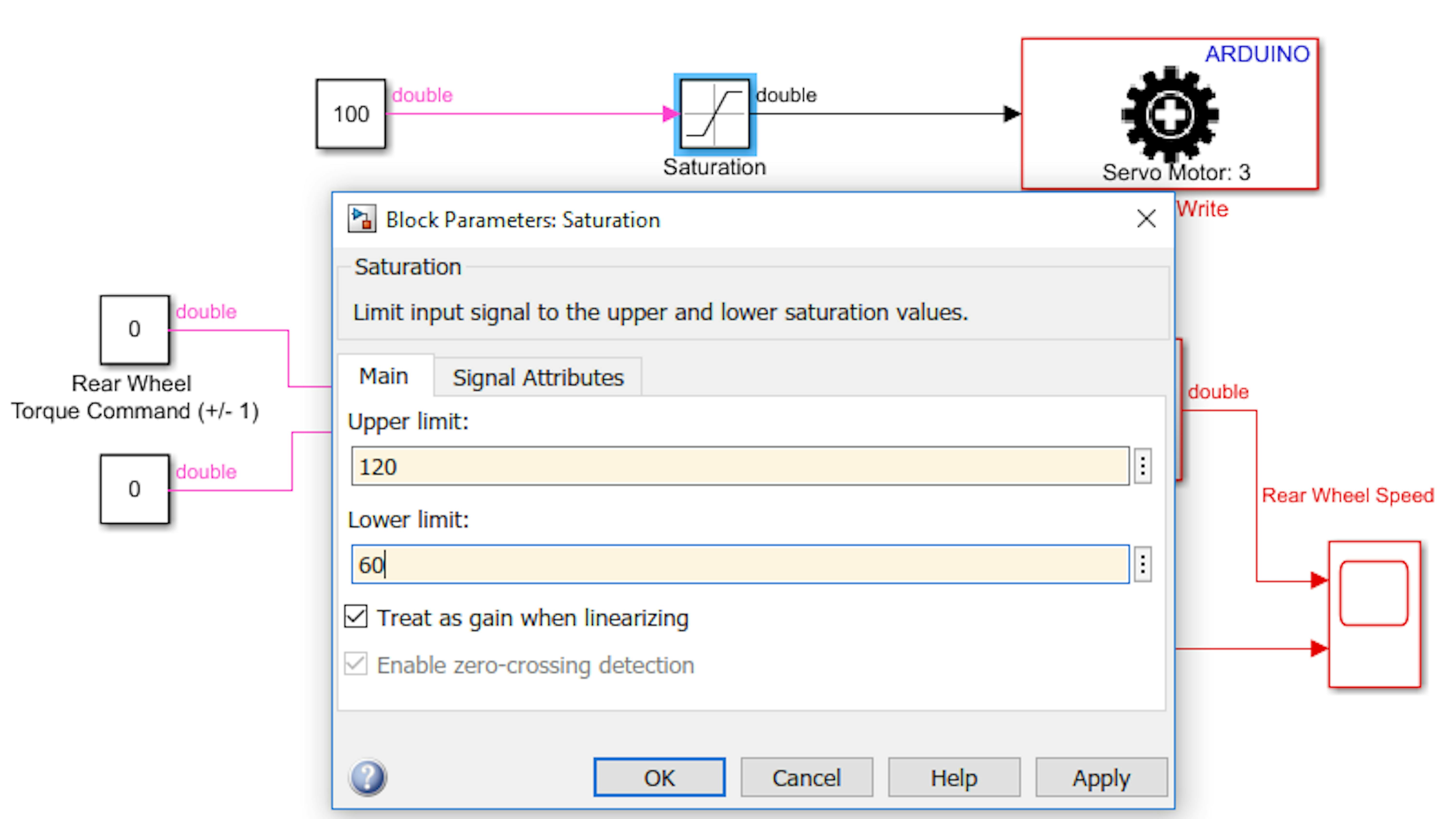
Now, find the angle at which the motorcycle’s front wheel is straight. This will require some trial and error. The value should be close to 90 but may be off depending on how precisely the steer column was fastened to the servo arm.
When you want the motorcycle to go straight, it is more intuitive to call that angle 0 rather than using the arbitrary value you just measured. You can then refer to left and right steer angles using positive and negative angles with respect to the “straight” servo angle. To do that, add a Bias block from Simulink → Math Operations and set the value to the “straight” servo angle you just measured:
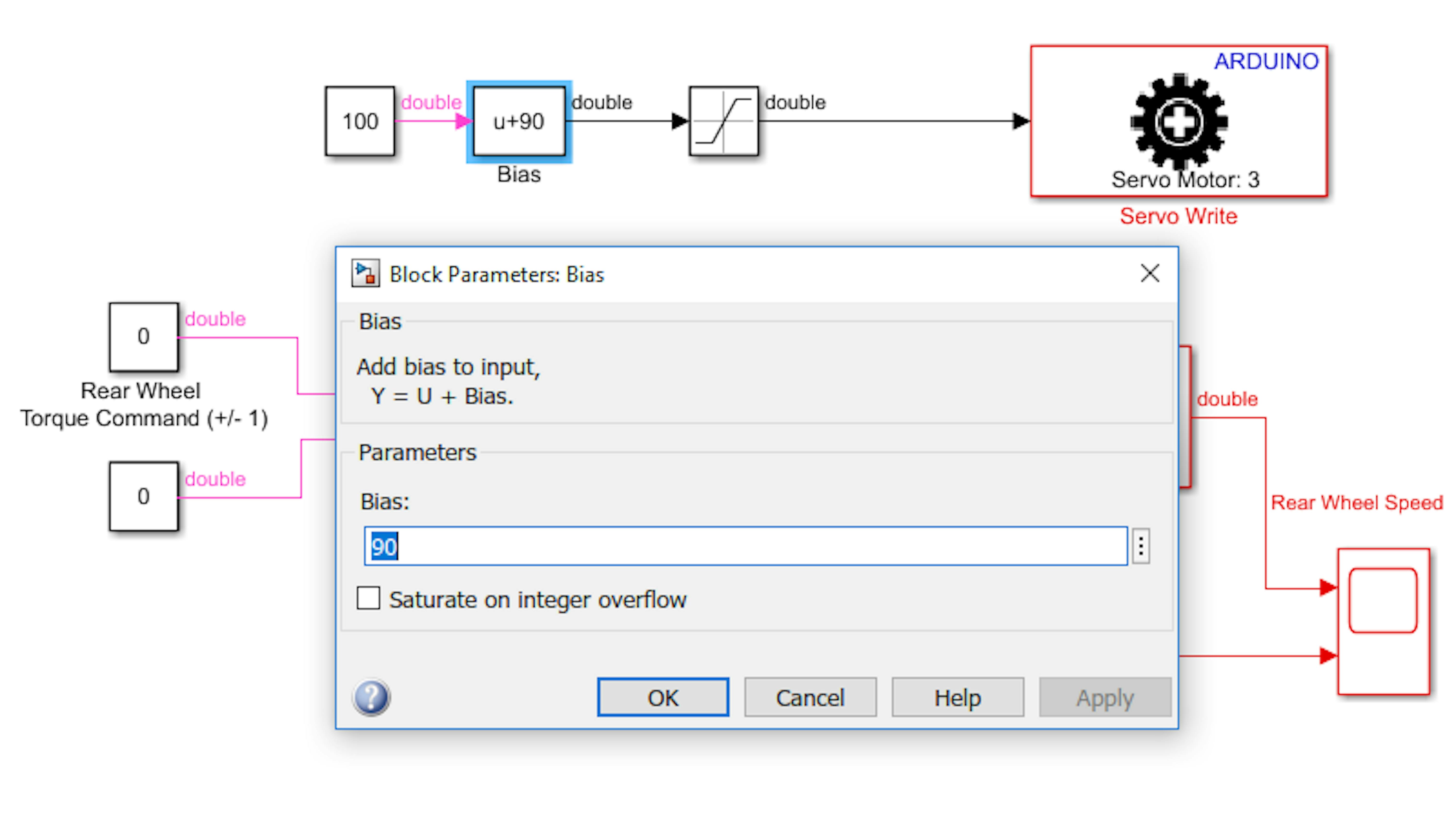
Now, set the Constant value to 0 and label the signals and blocks as shown:
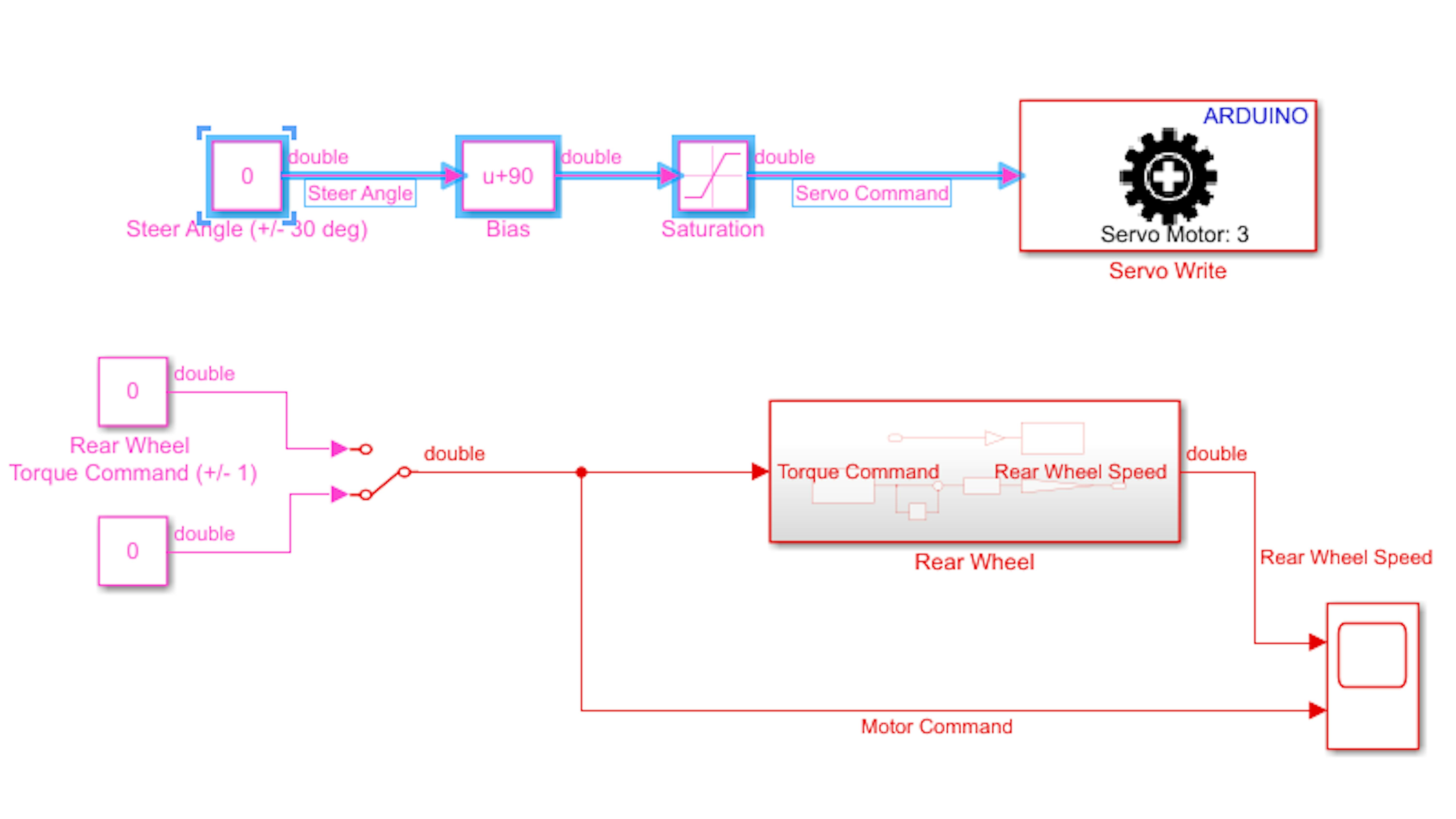
Run the model. Adjust the Constant value while the model is running. Ensure that a value of 0 points the steer column straight and positive and negative values give left and right steer angles, respectively. Also, make sure your saturation limits have taken effect (you should not be able to steer beyond approximately +/- 30 degrees).
Next, let’s clean up. Highlight the Bias, Saturation, and Servo Write blocks and create a subsystem for the steer servo:

Label the new subsystem block "Steer Servo" as shown:

Now, let’s make sure you can change the steer angle while the rear wheel is running. With the model still running, place the motorcycle’s kickstand in the vertical position:
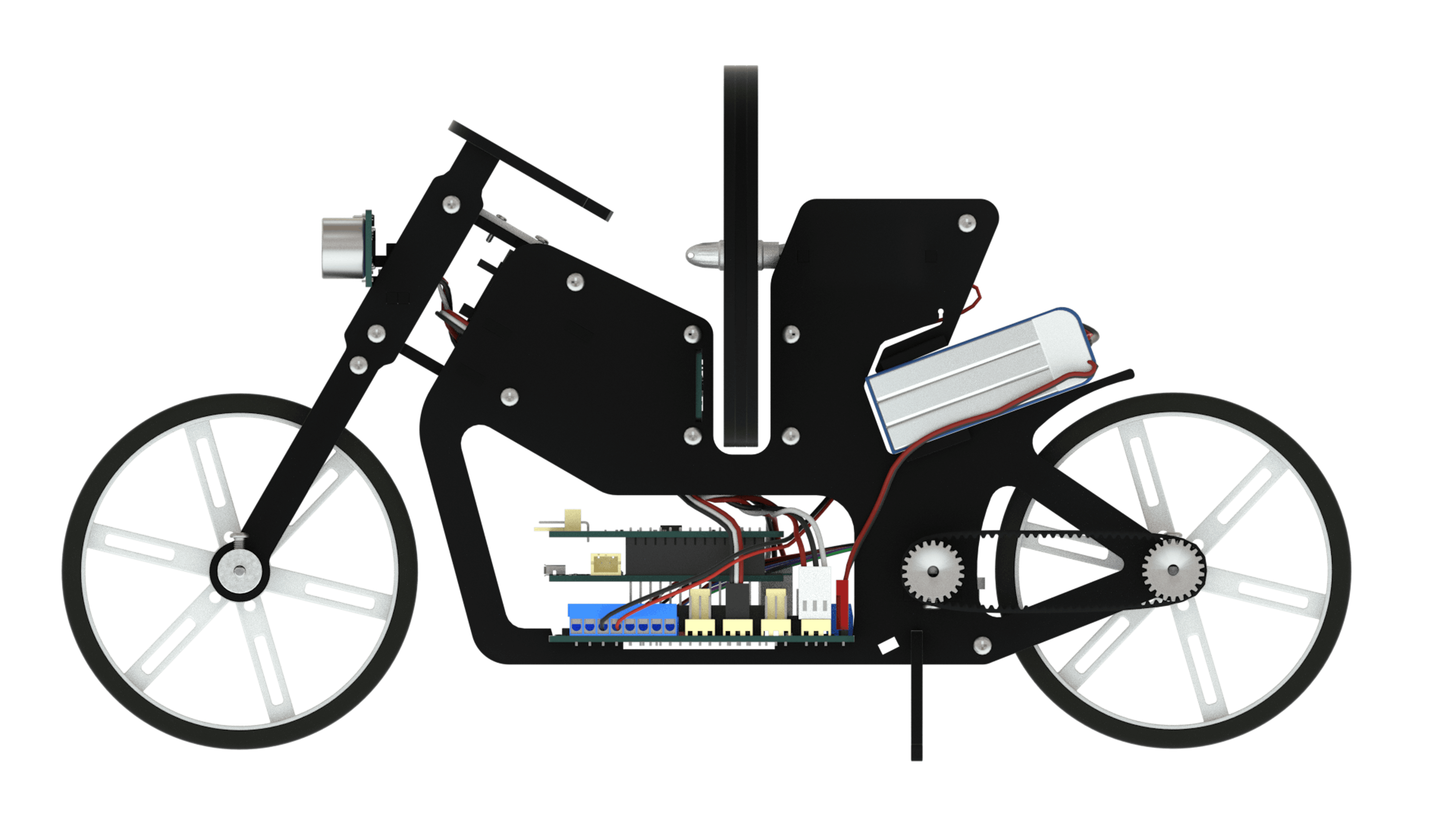
Enable the rear wheel using the manual switch. While the rear wheel is moving, try a few different steer angles using the new slider. Then, stop the rear wheel.
Restore the kickstand to its diagonal position:
Now, with the model still running, disconnect the USB cable from the motorcycle (the application should already be connected to your Wi-Fi network). Place the motorcycle on the ground and try adjusting the steer angle. Remember, to hold the motorcycle as it is moving because the balancing algorithm is not enabled here. Then, try driving forward or backward with varying speeds and steer angles.
When you are finished, stop the model.
BALANCING WITH SMALL STEER ANGLE
Next, you will attempt to balance the motorcycle while turning. To start, you will need to incorporate the servo motor algorithm into the system model. Open myNewMoto.slx.
Note: If myNewMoto.slx is incomplete or unavailable, open motoSys4_rWheel.slx and save it as myNewMoto.slx.
Copy the entire steer mechanism, consisting of the Steer Angle constant block and the Steer Servo subsystem, from myDrive.slx to myNewMoto.slx. You may need to move some signals around to make room:
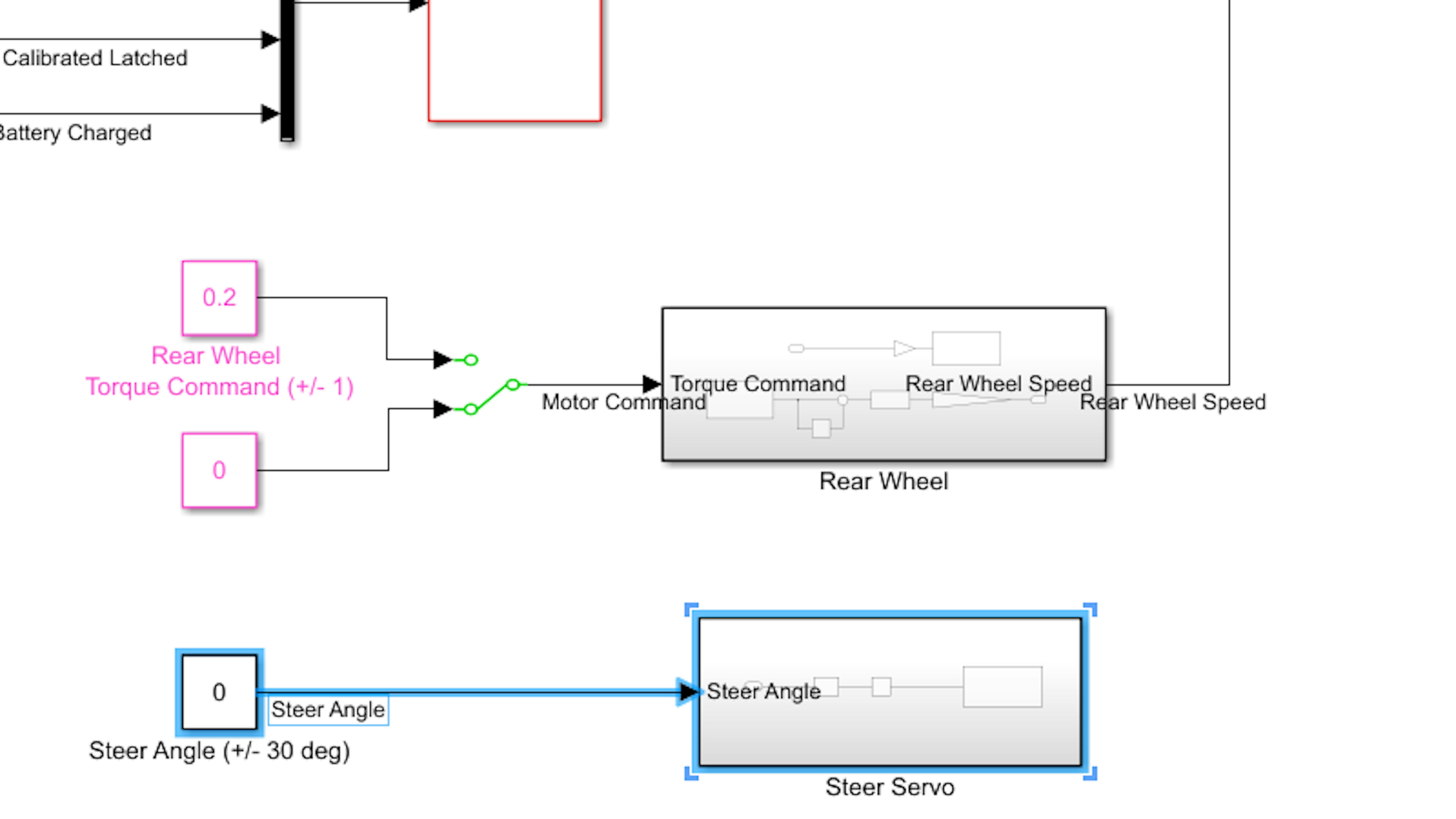
Now, create a branch off the Steer Angle signal and feed it into the Scope block, creating a third inport:
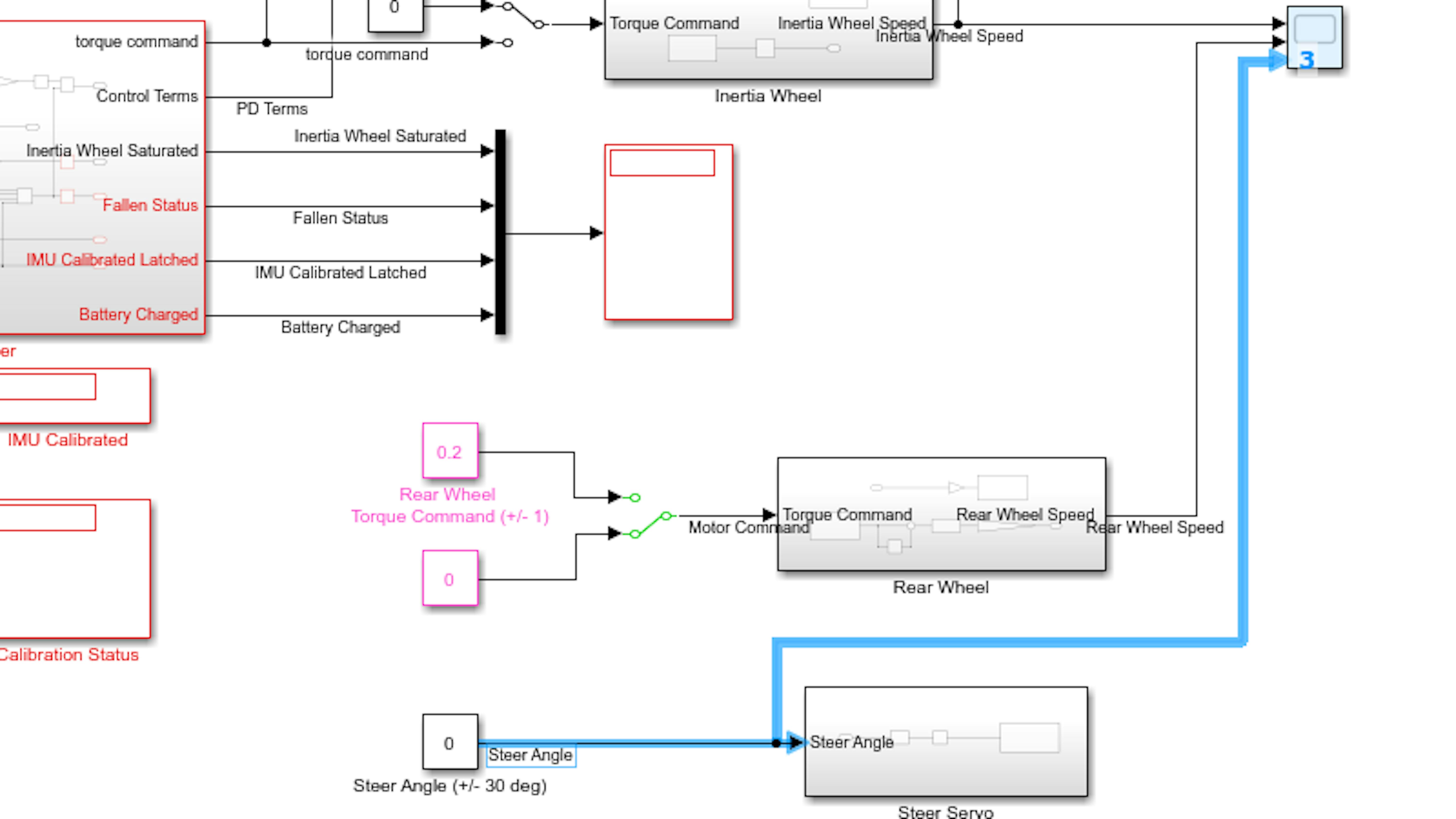
You are now ready to test the motorcycle’s balance while steering. Reconnect the USB cable between the motorcycle and your computer. Run the model and disconnect the USB cable from the motorcycle once the model is running. Calibrate the IMU as you have done before and make sure the bias is adjusted such that the balance point is close to θ = 0. Balance the motorcycle in place. Once you have it balancing in place, try adjusting the steer angle by changing the constant value (without rear wheel motion). Then, with the steer servo pointing straight, apply a small command to the rear wheel so that the motorcycle moves forward slowly. Once you can balance the motorcycle with straight motion, try a small turn, say, 5 degrees to the left or right.
Balancing on wide turns (small steer angles) may take some trial and error. If you are having trouble balancing, try decreasing the steer angle or decreasing the rear wheel speed. Both actions will decrease the centrifugal force acting on the motorcycle.
What happens to the inertia wheel speed when you are balancing the motorcycle throughout a turn? You will see that the inertia wheel must work extra hard while the motorcycle is turning to counteract the motorcycle’s inertia — its tendency to move in a straight line. You can reverse the inertia wheel’s acceleration by turning in the opposite direction.
:
As you can see, the motorcycle may balance for a shorter time while undergoing a wide turn, but it cannot continue turning indefinitely because the inertia wheel winds up, leading to a saturation shutdown or the motorcycle simply falling if the inertia wheel cannot generate enough torque to keep it vertical during a sharper turn.
To account for this effect, proceed to the final challenge, in which you will redesign the controller to lean into the turn so that the inertia wheel does not need to generate that extra torque.
LEARN BY DOING
In this chapter, you learned about the servo motor that controls the orientation of the motorcycle’s steer column. You then tested and calibrated the servo motor so that user inputs for the steer angle are expressed with respect to straight motion. Finally, you integrated the steer servo motor into the main system model and attempted to balance the motorcycle while turning at large radius.
When you change the steer angle, the servo motor abruptly moves the steer column from the initial angle to the final angle. For small increments in the steer servo angle, this is acceptable. However, for large increments in the steer angle, moving the steer column so fast can affect the stability of the balance controller. As an extra challenge, add some logic to the Steer Servo subsystem so that the maximum speed of the servo is limited. For instance, if you change the steer angle from -15 degrees to +15 degrees, it should take the servo motor, say, 2 seconds to make that transition (15 degrees/second) rather than nearly instantaneously. It will be up to you how you formulate the logic and what the maximum speed of the steer servo should be.
6.6 Lessons learned
In this chapter you were introduced to these following topics:
APPLY THE MATHEMATICAL THEORY IN THE SIMULINK MODEL
With the understanding of the motorcycle system dynamics you have learned how to apply the equations of motion to act on the inertial wheel and counterbalance its tendency to fall. To do this, you used a simulation of a 3D model whose behaviour is determined by Simulink blocks.
PID CONTROL MODELING BASED ON IMU SENSOR DATA
You also learned how to build your PID control system, using the positioning sensor data to feed the control algorithm, and studied how the PID controller responds to different random stimuli and which factors (Kp, Ki, and Kd) matter the most to keep the motorcycle standing.
APPLY SAFETY MEASURES
You learned how to integrate different safety measures into your system to protect your hardware from damaging. The safety measures includes battery protection, deactivation of inertial wheel when the motorcycle loose balance, limitation of the inertial wheel speed using a tachometer and stopping the system from running until the IMU is calibrated.
WIRELESS COMMUNICATION
You also learned how to configure the communication with the MKR1000 to send data via WiFi. In this manner you are capable of controlling the motorcycle remotely by sending commands like turning, steering, increasing speed or changing the motor direction.
6.7 Final challenge: Executing coordinated banked turns
For the final challenge of the motorcycle project, you will modify the controller algorithm so that the motorcycle leans inward as it turns. You probably do this instinctively when you ride a bicycle (or drive a life-sized motorcycle). For 2-wheeled vehicles, it is necessary to lean inward while turning for stability. In this final challenge, you will learn about the mechanics of a turning motorcycle, identify the optimal lean angle for turns, and adjust the controller algorithm so that the motorcycle tends towards the optimal lean angle at all times.
In this exercise, you will learn the following:
- Understand the physical mechanics of a turning motorcycle.
- Derive the optimal lean angle to minimize motor torque during turns.
- Configure the system model to calculate the optimal lean angle from the motorcycle speed and the steer angle.
- Redesign the balance control algorithm to lean at the optimal angle while turning.
- Balance the motorcycle while turning at arbitrary speeds and turn radii without expending excessive torque in the inertia wheel motor.
FINDING OPTIMAL LEAN ANGLE DURING TURNS
To understand why the motorcycle must lean into turns to keep the inertia wheel from ramping up, let’s look at the following diagram in which we are viewing the motorcycle from behind as it is turning left:
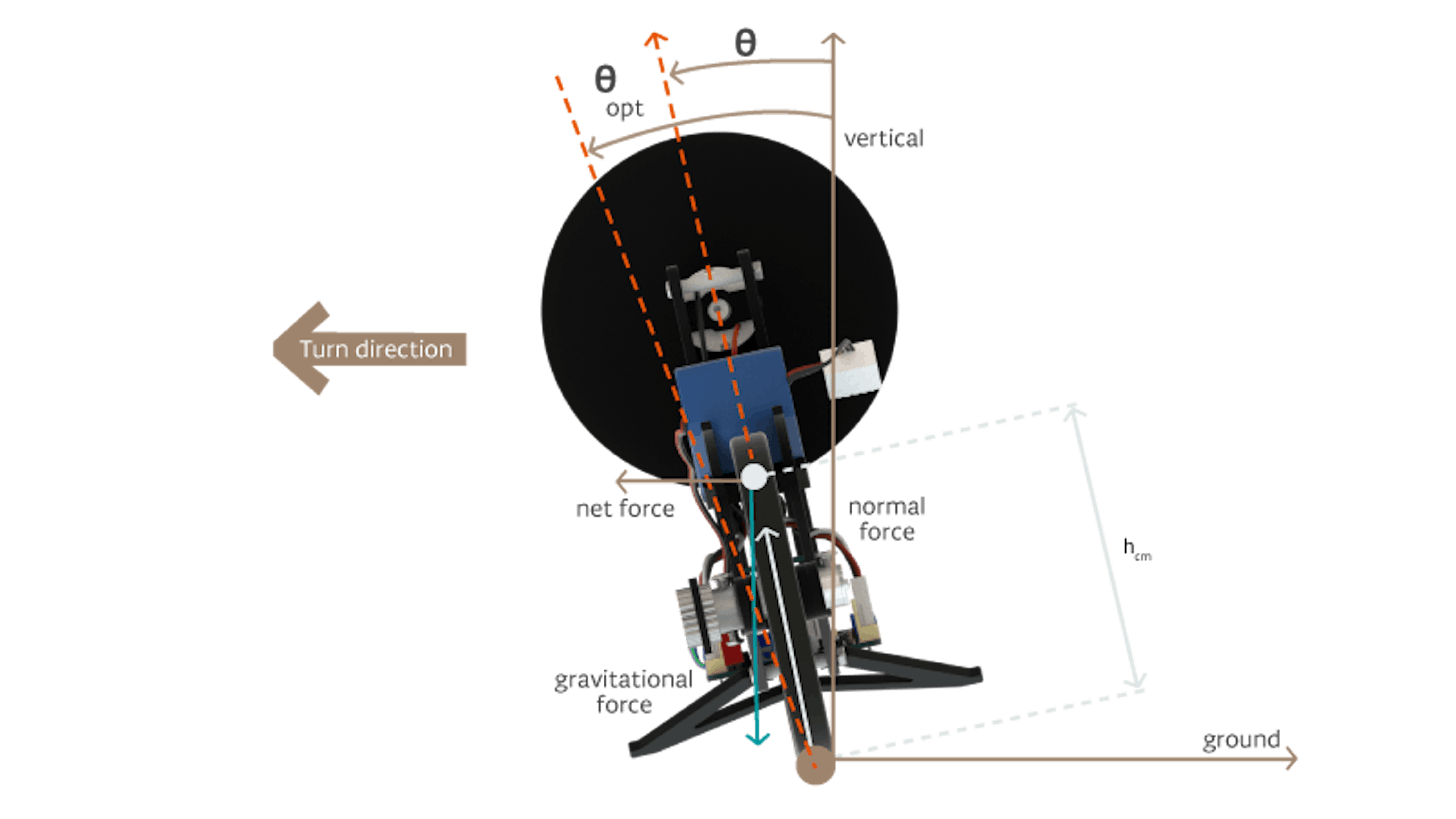
Consider the torques acting on the motorcycle about the wheel-ground axis. We will consider the moving motorcycle frame, in which all forces and torques are expressed from the motorcycle’s perspective. As usual, there is a gravitational torque due to the gravitational force acting on the motorcycle’s center of mass. This torque gets larger when the motorcycle leans farther out from the vertical plane since the force acts farther from the rotational axis. Recall the formula for the gravitational torque:
$\tau_{g,M} = M_M\cdot g\cdot h_{cm}\cdot\sin(\theta)$
Here, $M_M$ is the mass of the motorcycle, including the inertia wheel and electronics, g is the constant gravitational acceleration, $h_{cm}$ is the height of the motorcycle’s center of mass from the wheel-ground axis, and θ is the lean angle of the motorcycle, where a positive value is defined to be counterclockwise when viewed from behind.
When the motorcycle turns, it also experiences a centrifugal force (with respect to the motorcycle frame), which pulls the motorcycle outward from the turn direction. You have experienced a centrifugal force when riding in a car that is turning. When the car turns left it feels as though you are being pushed against the right side of the car. This is really a frictional force. What is really happening is that when you are in a turning car, your reference frame is accelerating inward, relative to the fixed ground frame. When you are in an accelerating reference frame, you feel a force acting on you in the opposite direction of that acceleration. However, it is perfectly valid to consider the physical mechanics with respect to any reference frame you wish.
The centrifugal force acts on the motorcycle’s center of mass against the turn direction (i.e. the centrifugal force pulls left when the motorcycle turns right). When the motorcycle leans at an angle θ, the center of mass lies $h_{cm}{\cdot}cos(\theta)$ above the rotational axis. Therefore, the centrifugal torque on the motorcycle with respect to the wheel-ground axis is:
$\tau_{centrifugal,M} = -M_M{\cdot}\frac{V^2}{R_{turn}}{\cdot}h_{cm}{\cdot}\cos(\theta)$
In the above equation, V is the speed of the motorcycle (forward or backward) and $R_{turn}$ is the turn radius, defined as the radius of the circle traced by the motorcycle as it turns. The centrifugal torque increases when it turns at a sharper radius (smaller $R_{turn}$) or a faster speed. What if the motorcycle is not turning? In this case, the turn radius goes to infinity, and thus, the centrifugal torque is 0.
Next, let’s consider the net torque on the motorcycle in its own reference frame. We have previously discussed gravitational and centrifugal torque. There is also the torque of the inertia wheel pushing against the motor shaft, as discussed in exercise 6.1, $\tau_{W,M}$. Finally, any other torques from the environment, such as bumps in the road or drag, are accounted for in $\tau_{ext,M}$. Together, we have the net torque on the motorcycle with respect to the wheel-ground axis:
$\tau_{net,M} = \tau_{g,M} + \tau_{centrifugal,M} + \tau_{IW,M} + \tau_{ext,M}$
To find the equilibrium lean angle, where the motorcycle is perfectly balanced (albeit unstably), we will assume the motor is turned off, and therefore, the inertia wheel is not pushing against the motor shaft:
$\tau_{IW,M} = 0$
We will also assume there is no external torque beyond the gravitational and centrifugal torques:
$\tau_{ext,M} \approx 0$
This gives an unmotorized net torque as follows:
$\tau_{net,M,no\ motor} \approx \tau_{g,M} + \tau_{centrifugal,M}$
$= M_M{\cdot}g{\cdot}h_{cm}{\cdot}\sin(\theta) - M_M{\cdot}\frac{V^2}{R_{turn}}{\cdot}h_{cm}{\cdot}\cos(\theta)$
When the motorcycle is in equilibrium, the unmotorized net torque is equal to zero:
$\tau_{net,M,no\ motor}(\theta_{opt}) \approx M_M{\cdot}g{\cdot}h_{cm}{\cdot}\sin(\theta_{opt}) - M_M{\cdot}\frac{V^2}{R_{turn}}{\cdot}h_{cm}{\cdot}\cos(\theta_{opt}) = 0$
In the above equation, $\theta_{opt}$ is the optimal lean angle, at which the net torque is 0. Solving for $\theta_{opt}$, we have:
$\theta_{opt} = \tan^{-1}(\frac{V^2}{R_{turn}{\cdot}g})$
If we tell the controller to move the lean angle to $\theta_{opt}$ while it turns rather than maintaining θ = 0, then the inertia wheel motor will not have to exert extra torque to counteract the centrifugal torque. This will allow for more realistic and power-friendly exertion by the motor.
In the equation above, we already know how to measure the motorcycle speed V from the rear wheel encoder. Now, we need to figure out how to get the turn radius, $R_{turn}$. Consider the following diagram:
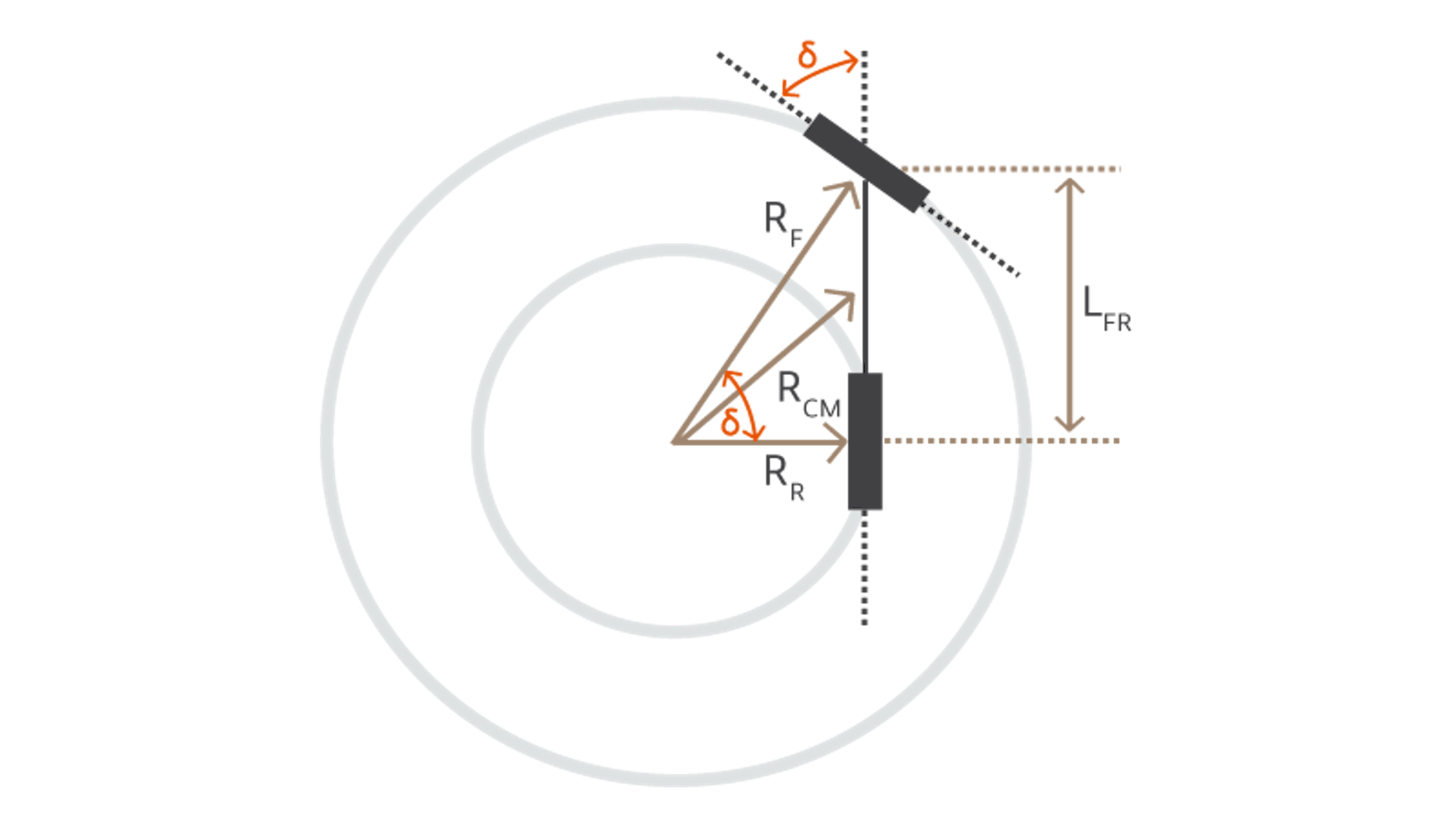
In the above picture, we are looking at the motorcycle from above. When the front wheel is turned, we can imagine 2 concentric circles that lay tangent to the front and rear wheels. Let’s call the steer angle δ. When the motorcycle turns with a constant steer angle, the front wheel traces a larger circle than the rear wheel. The distance between the centers of the front and rear wheels is $L_{FR}$, and the respective radii of the circles are $R_{F}$ and $R_{R}$.
The two circle radii form a right triangle with the wheel-ground axis. The angle between the front and rear wheel radii is equal to the steer angle δ. Using trigonometric relationships, we have:
$R_F = \frac{L_{FR}}{\sin(\delta)}$
$R_R = \frac{L_{FR}}{\tan(\delta)}$
The centrifugal force acts at the center of mass of the motorcycle. It is generally somewhere between $R_F$ and $R_R$. Now, considering only small steer angles, we can make the following approximation:
$R_F \approx R_R \approx R_{cm} \approx \frac{L_{FR}}{\delta}$
Now, substituting this radius for $R_{turn}$ in the equilibrium angle $\theta_{opt}$, we have:
$\theta_{opt} \approx \tan^{-1}(\frac{V^2{\cdot}\delta}{L_{FR}{\cdot}g})$
We have now expressed the target lean angle in terms of measurable quantities. You have control of the steer angle δ through the steer servo, and you can adjust the motorcycle speed V using the rear wheel torque command. The rear wheel-front wheel distance $L_{FR}$ is easily measurable. And in most cases, g will be equal to $9.81 m/s^2$ (though the motorcycle should work just as well on other planets with proper adjustment of g!).
Now let’s look at a Simulink model that incorporates the centrifugal torque in the physical dynamics. Open the model motoSys1b_centrifugal.slx:
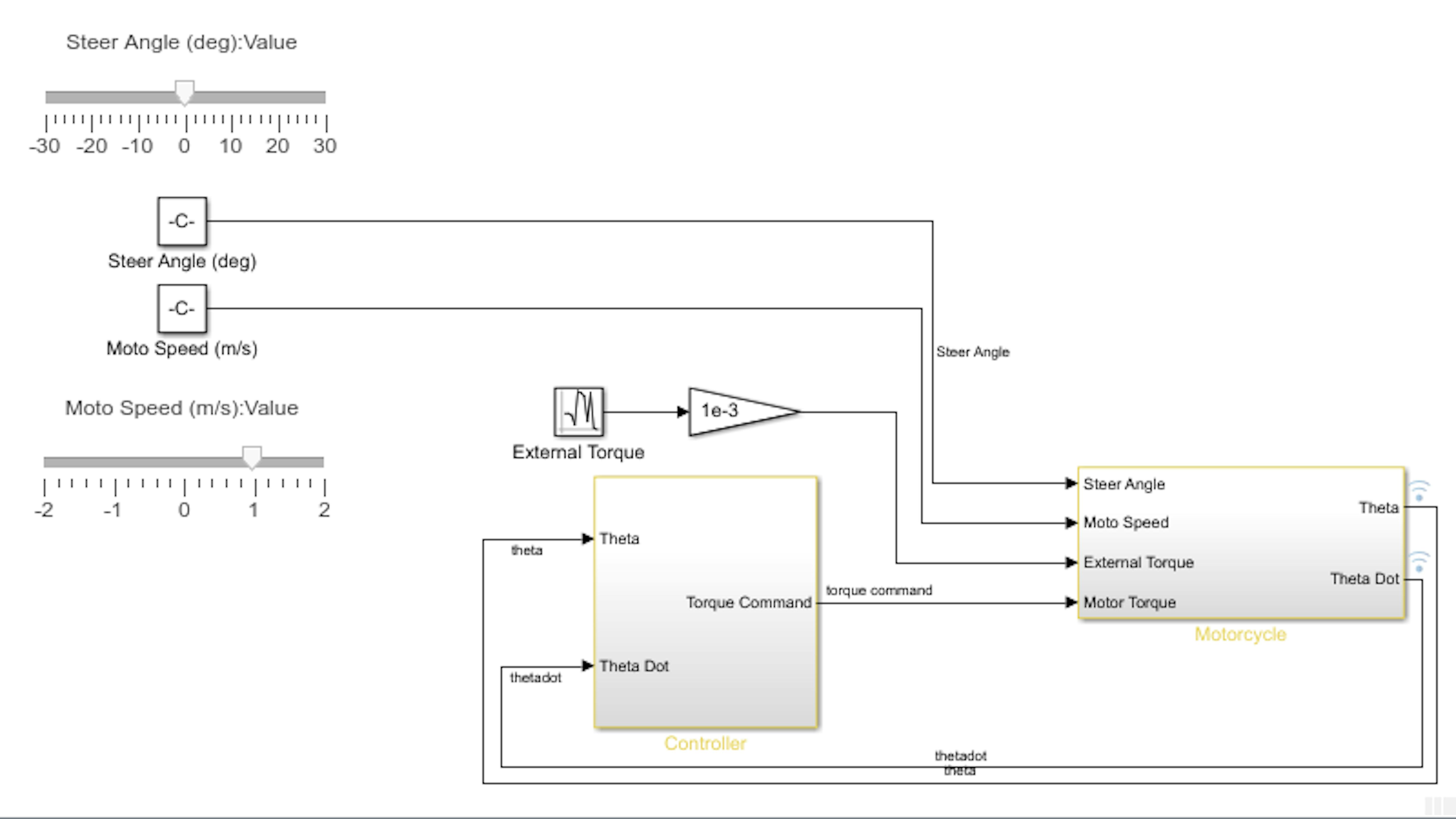
Examine the model. This model is similar to the one you used in Exercise 6.1. The Motorcycle subsystem contains SimScape blocks that implement the differential equations of the physical system. However, this time, there are additional inputs to the Motorcycle subsystem for the steer angle command and the motorcycle’s forward speed.
Now, run the model and watch the animation play in the Mechanics Explorers window as the model runs:
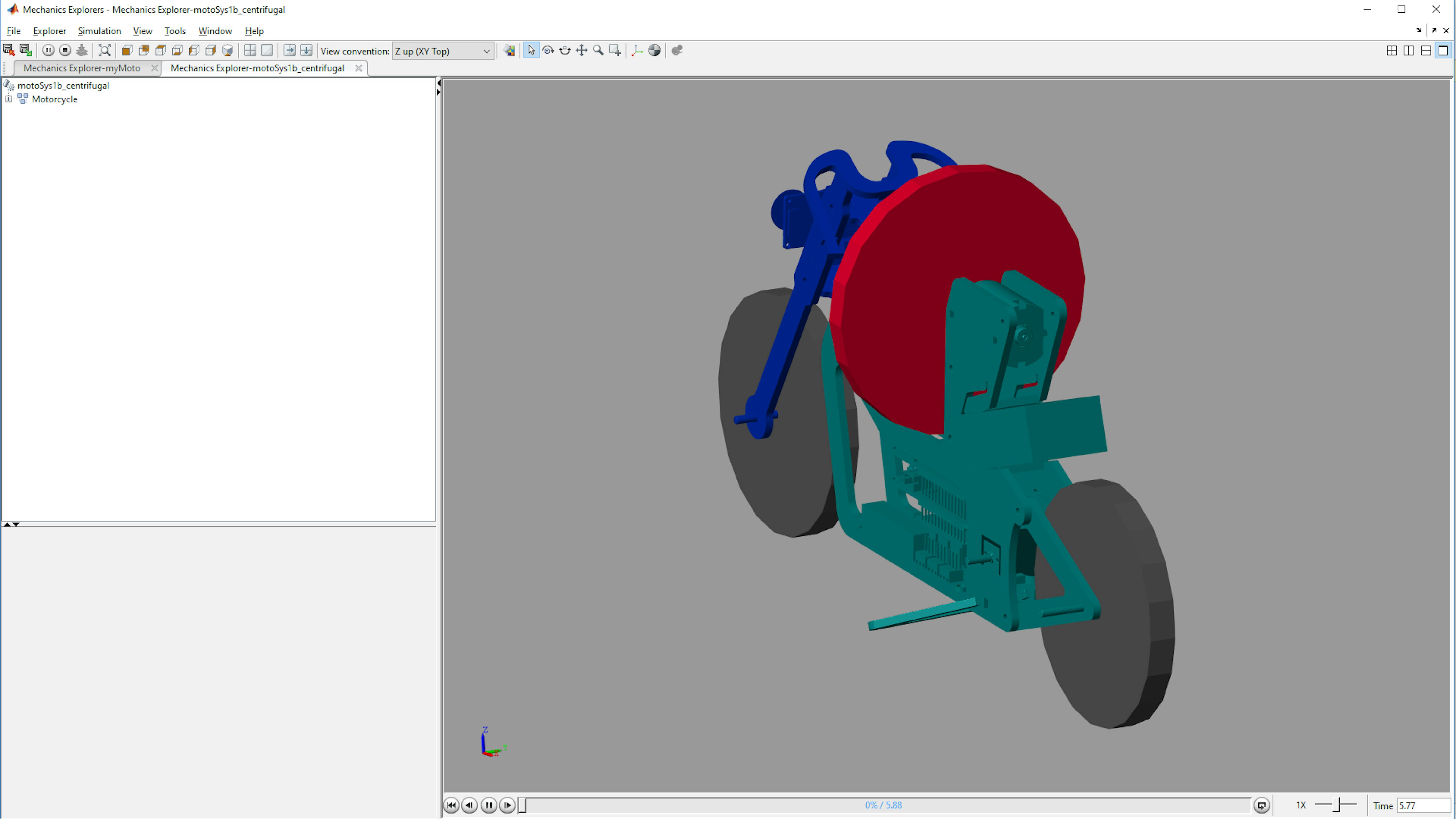
Try adjusting the steer angle using the slider in the model and watch what happens in the animation. You will see that when you turn the motorcycle, the motorcycle perturbs in the opposite direction and then attempts to restore itself to θ = 0. As of now, we haven’t changed anything about the controller algorithm. It is always trying to bring itself to θ = 0, even if it is turning and could expend less energy by leaning into the turn.
To formally observe the motorcycle’s behavior, open Simulation Data Inspector (SDI) using the  button in the model window. As the model is running, examine the torque command and Steer Angle signals in SDI:
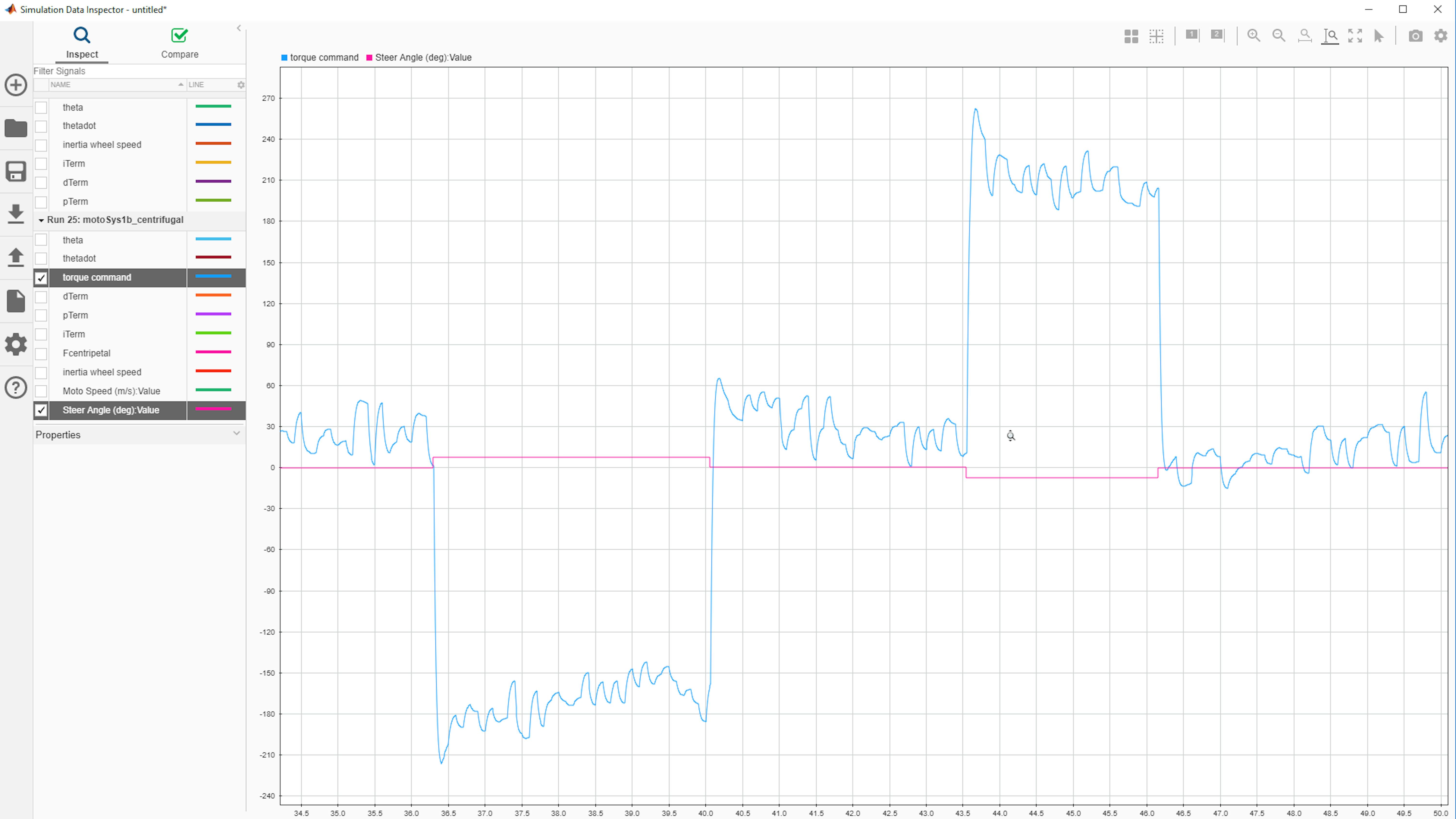
Here, you can see the motor trying to counteract the centrifugal force during turns.
Next, examine the torque command and inertia wheel speed signals:
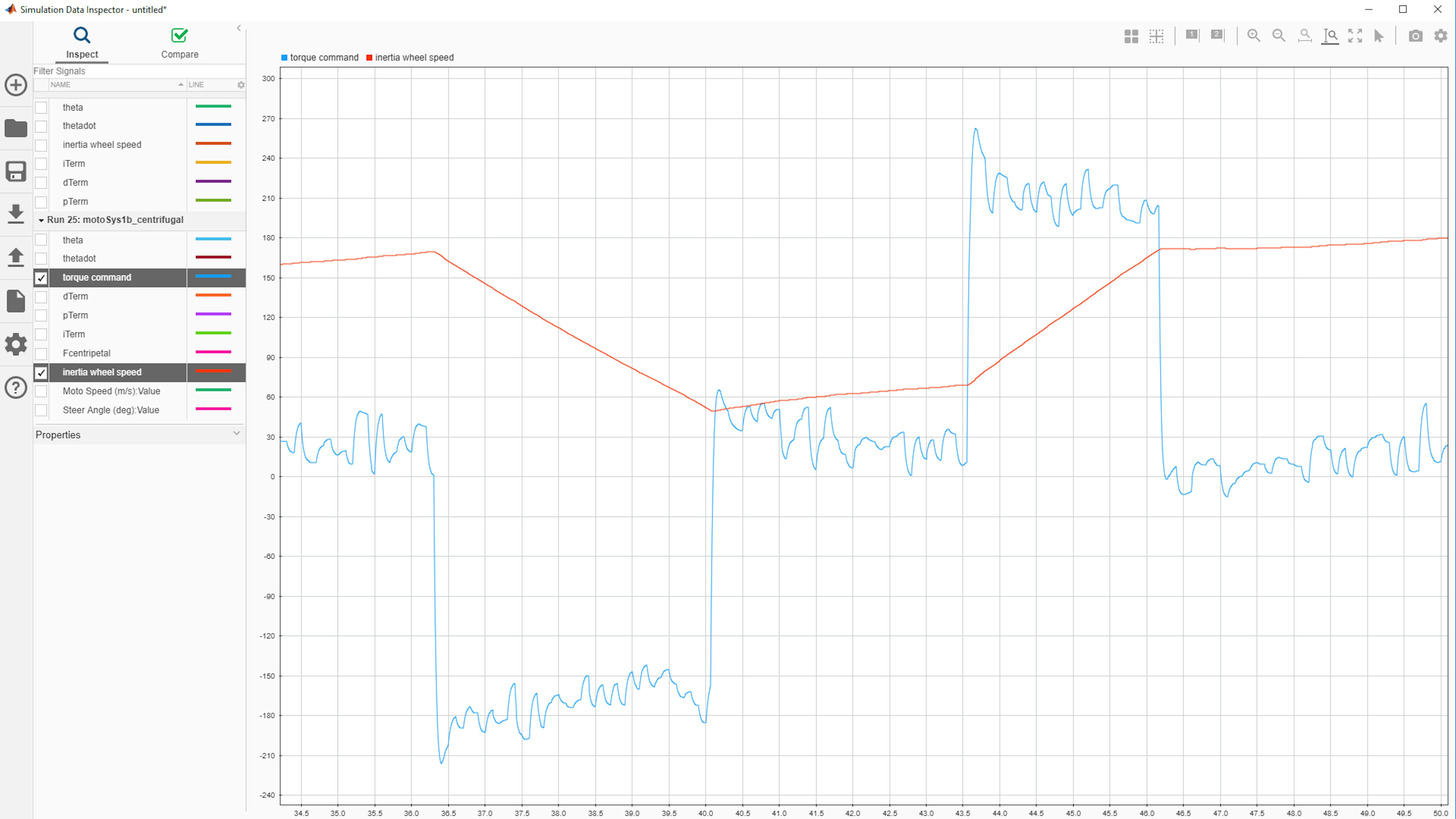
Notice how the inertia wheel accelerates continuously during the times when the motor is correcting for a centrifugal force. After gaining some experience working with the motorcycle hardware, you can fully appreciate how unrealistic this behavior would be to implement on the real motorcycle.
Finally, examine the Steer Angle and theta signals:
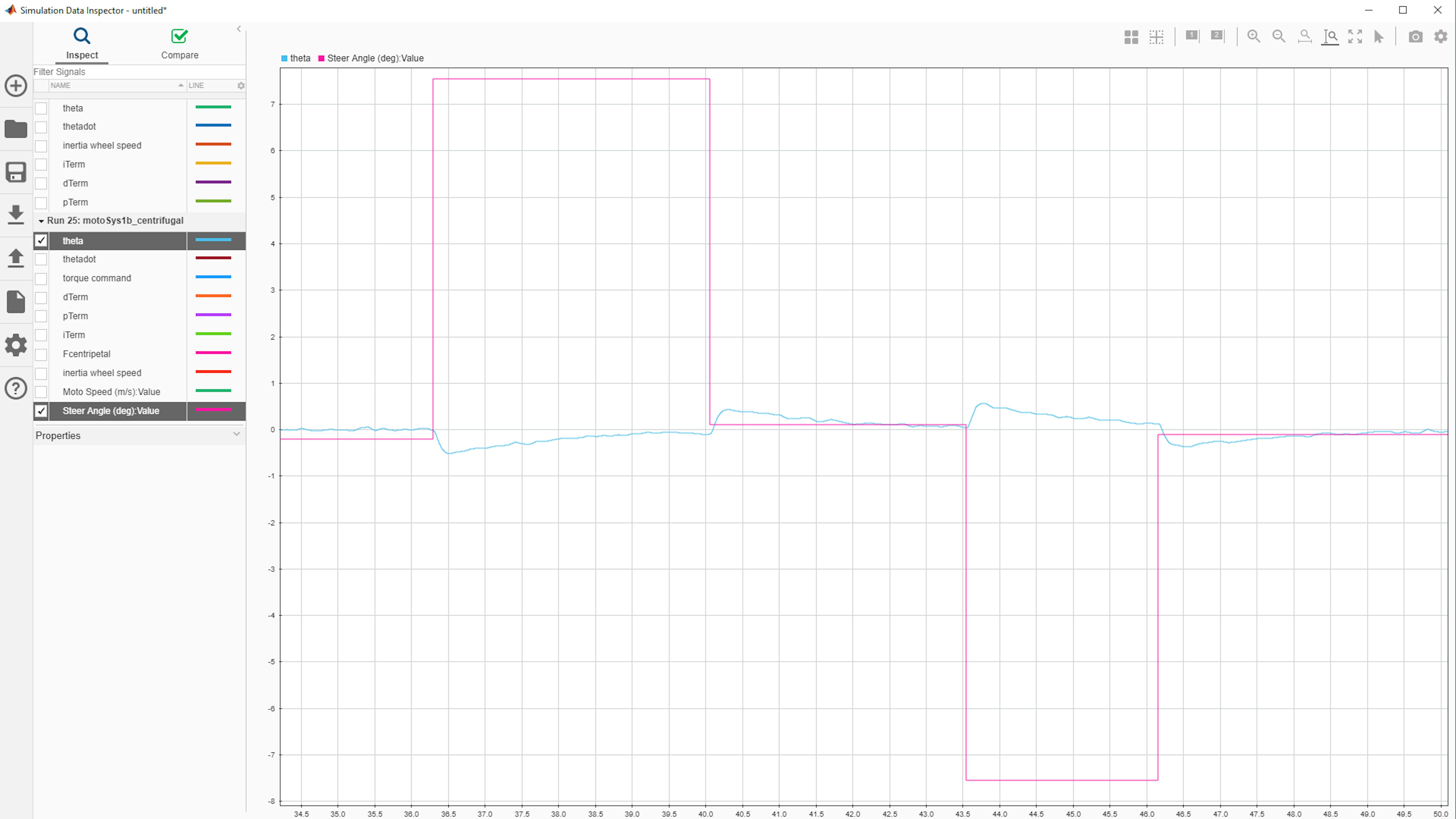
Notice how the lean angle is always aiming for 0 degrees rather than the optimal lean angle for a given turn.
THE CHALLENGE
For your final challenge, you will attempt the following tasks:
- In motoSys1b_centrifugal.slx, add logic to calculate the optimal lean angle ($\theta_{opt}$) as a function of the steer angle and the motorcycle speed (use the equations at the beginning of this exercise as a guide).
- Modify the controller algorithm in motoSys1b_centrifugal.slx so that the controller pushes the motorcycle toward θ = $\theta_{opt}$, instead of θ = 0.
- Simulate the modified control algorithm in Normal mode and use Mechanics Explorer and Simulation Data Inspector to confirm that the motorcycle leans correctly during turns and the inertia wheel speed remains low during turns.
- Starting with myNewMoto.slx (or motoSys5_steer.slx), make the same modifications to the controller algorithm so that the motorcycle performs coordinated banked turns. Use the Rear Wheel Speed signal to get the motorcycle’s forward speed and use the Steer Command signal to get the turning angle.
- Run the model on the motorcycle’s MKR1000 board.
- Test the motorcycle’s balance during turns with various speeds and steer angles.