
DRAWING ROBOT
Drawing Robot
In this project, you'll build a robot that can draw on a whiteboard. When you are done, your robot will be able to acquire an image of a whiteboard (or load an existing image), extract the line traces from that image, scale the drawing to the drawable area of your whiteboard, and then reproduce the drawing by moving a marker along the same set of paths. Along the way, you'll learn important concepts in engineering, physics, and programming that are useful for a wide variety of applications.
In the exercises that make up this project, you will learn to:
- Connect to an Arduino-based robot from MATLAB
- Write MATLAB apps, functions, and scripts to control your robot
- Learn and apply concepts from geometry, physics, symbolic math, and image processing
- Automate a complete application workflow from start to finish
By the time you are ready to start with the coding, you should have assembled the robot following the instructions you can see below:
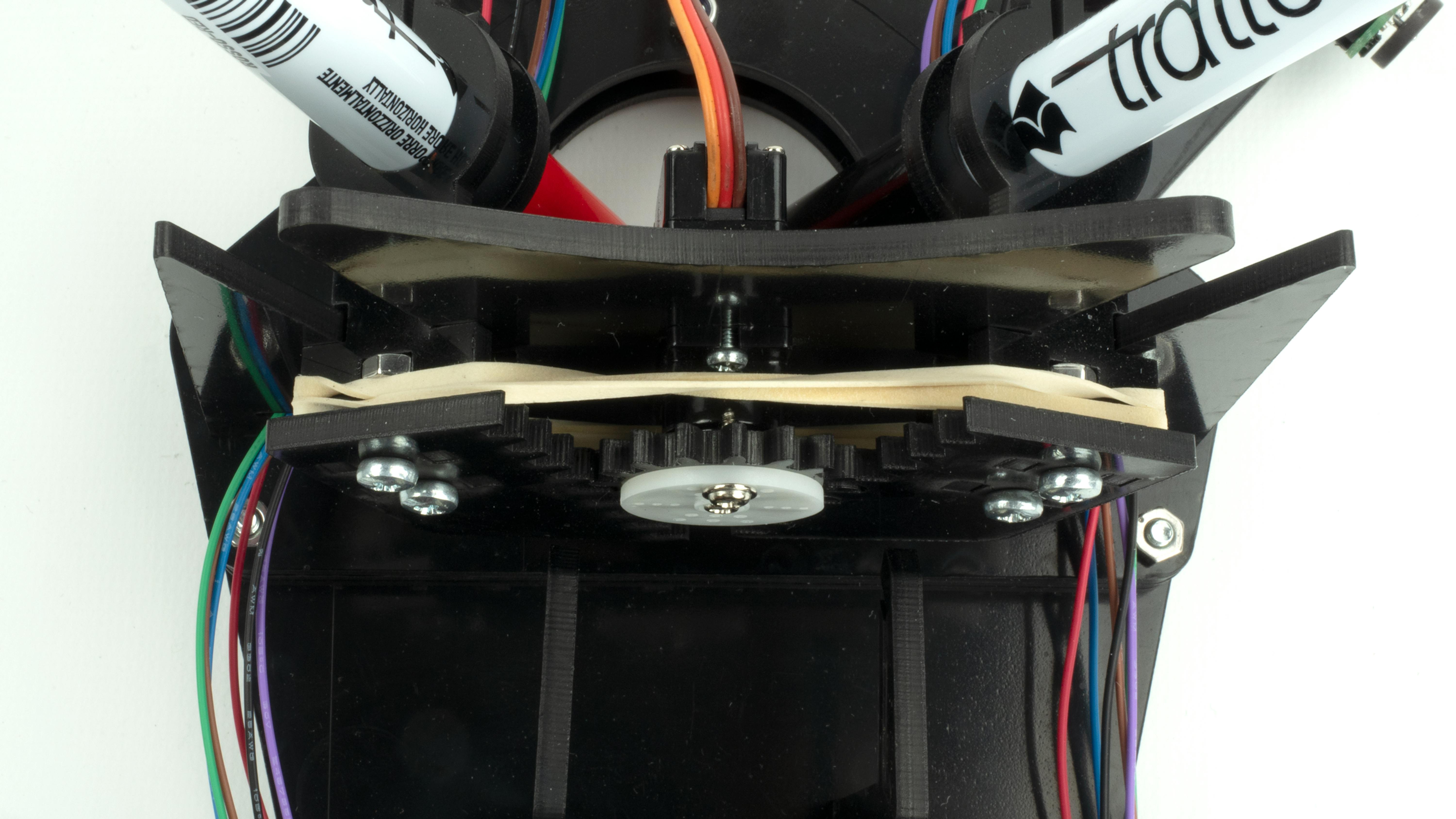
If you observe that cogwheel is skipping steps or getting jammed, you can use a rubber band on the pen holder pieces around the servo. In our tests, we found that using only one of the provided rubber bands and double wrapping the pieces worked reliably well.
EXERCISE 1 :
4.1 Introduction to the Drawing Robot
Once you have assembled the robot, you'll want to connect to your robot and make sure you can control all its parts. This exercise introduces all the commands needed to do so.
In this exercise, you will learn to:
- Connect to assembled robot
- Communicate with the robot's various components
CONNECT TO THE ROBOT
Let's get connected to the robot. You'll connect to your robot the same way you did in the Getting Started section. Connect the MKR1000 to your computer and run the arduinosetup command at the MATLAB command prompt. This will launch the Arduino hardware setup interface.
>> arduinosetup
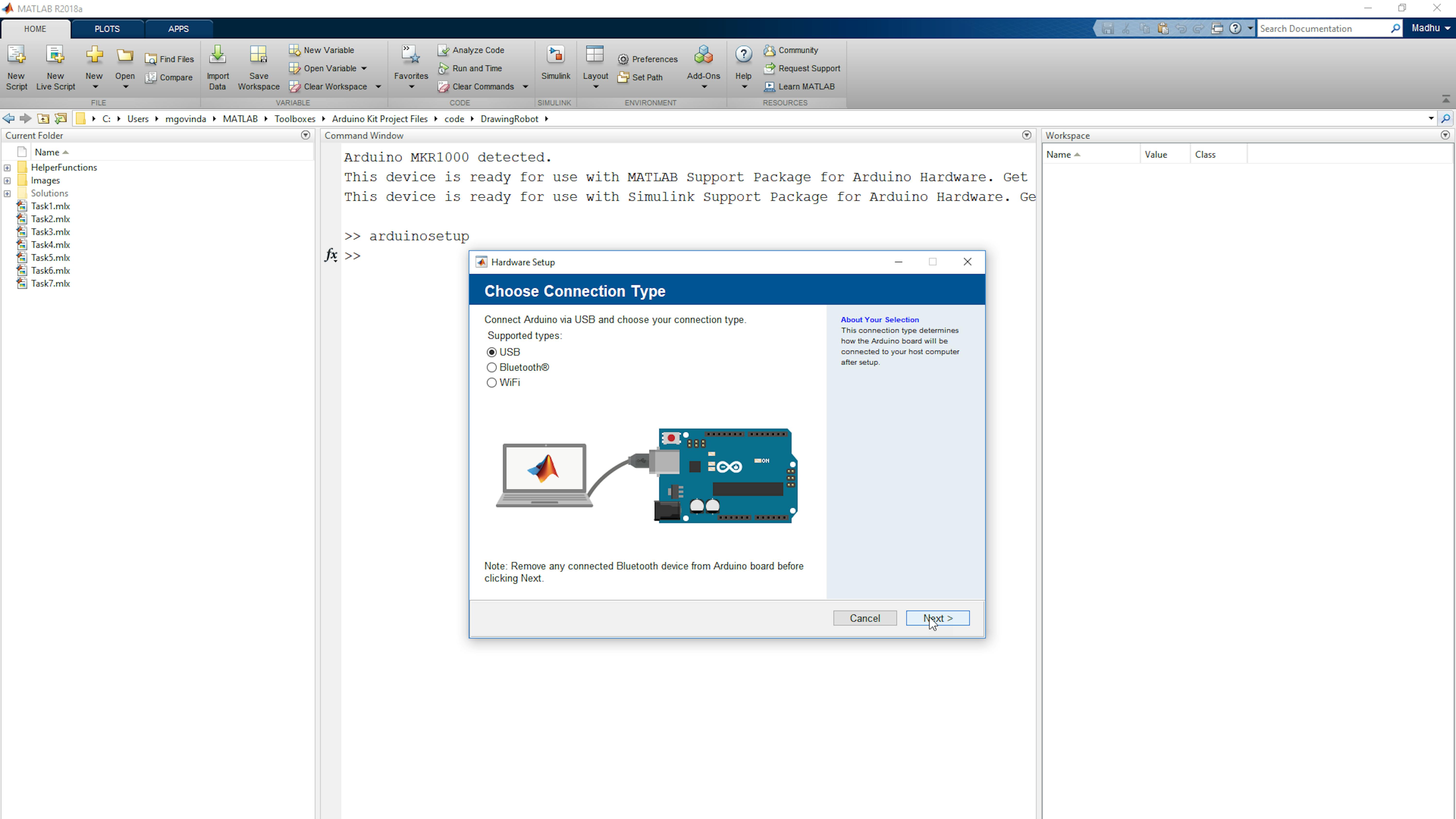
Select USB. Click Next. On the following screen, include the Arduino/MKRMotorCarrier library as well as I2C, SPI, and Servo. From the Port dropdown list, choose the port that the Arduino is connected to (COM## for Windows, /dev/ttyACM## for Linux, /dev/tty.usbmodem## for OSX). Click Program to upload the program to the board.
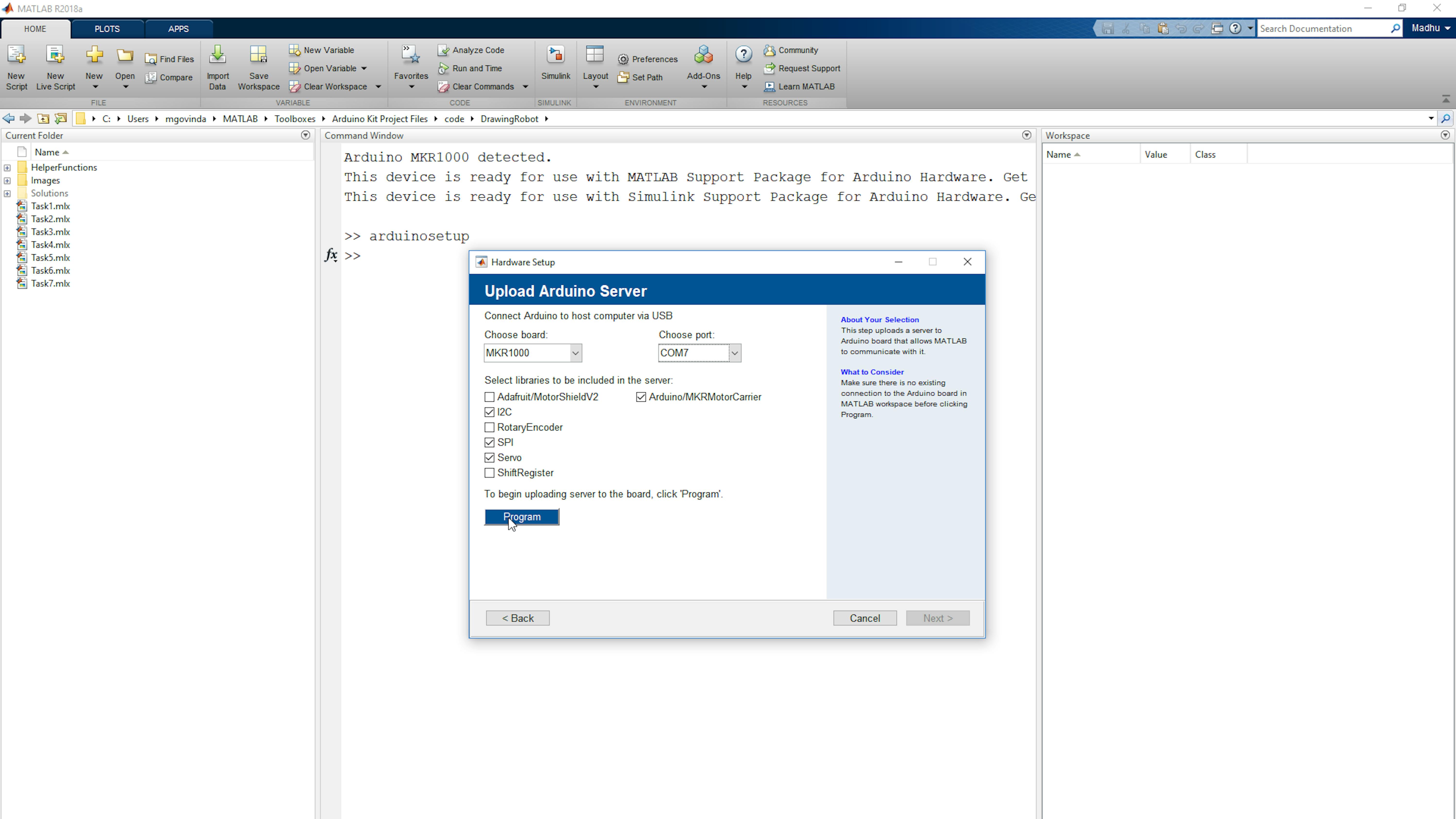
Note: This may take several minutes. If you receive an error message related to source not being found for the Arduino/MKRMotorCarrier library, then type edit ArduinoKitHardwareSupportReadMe.txt in MATLAB Command Window and follow the instructions provided on this text file.
Once the upload is complete, test the connection on the next screen using the Test Connection button. Close the setup interface.
CONNECT TO THE HARDWARE
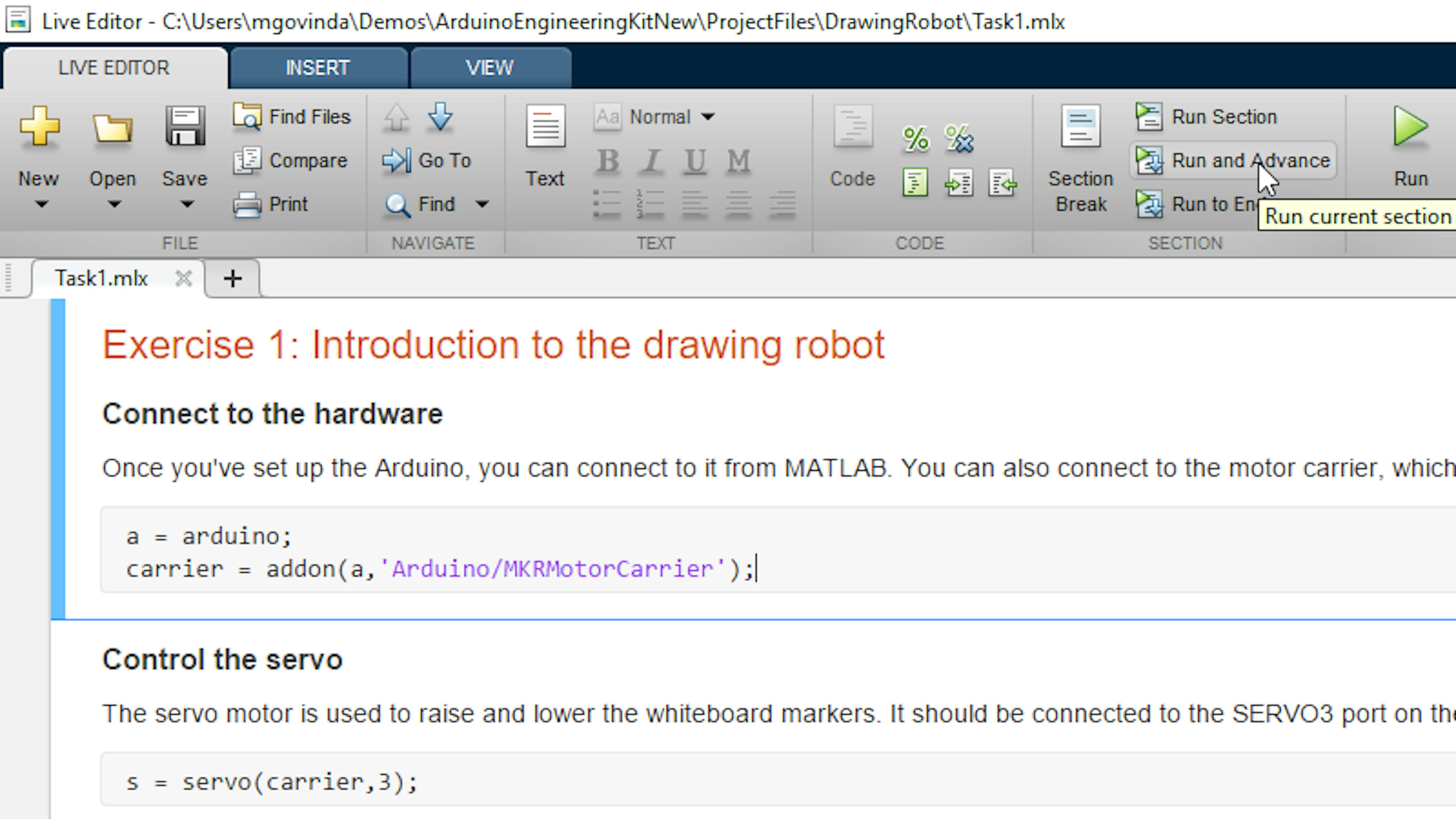
First, you will connect to the Arduino board from MATLAB. Open the live script, Task1.mlx by typing:
>> edit Task1Then, run the code in the Connect to the hardware section.
CONTROL THE SERVO
The drawing robot has two different color markers that can be raised and lowered by means of a servo motor. In this section, you will learn how to estimate the software limitations for driving the motor, given the physical limitations of the robot.
You need to be able to communicate with the servo motor and command it to raise and lower the two markers. This is a trial and error process where you'll need to experiment to determine the servo positions that lower the markers without trying to drive the motor beyond the limits of the marker channels.
The Task1.mlx live script contains code for you to connect to the servo motor and command it to move. First, connect to the motor by running the sections under the heading. Control the servo in the live script Task1.mlx.
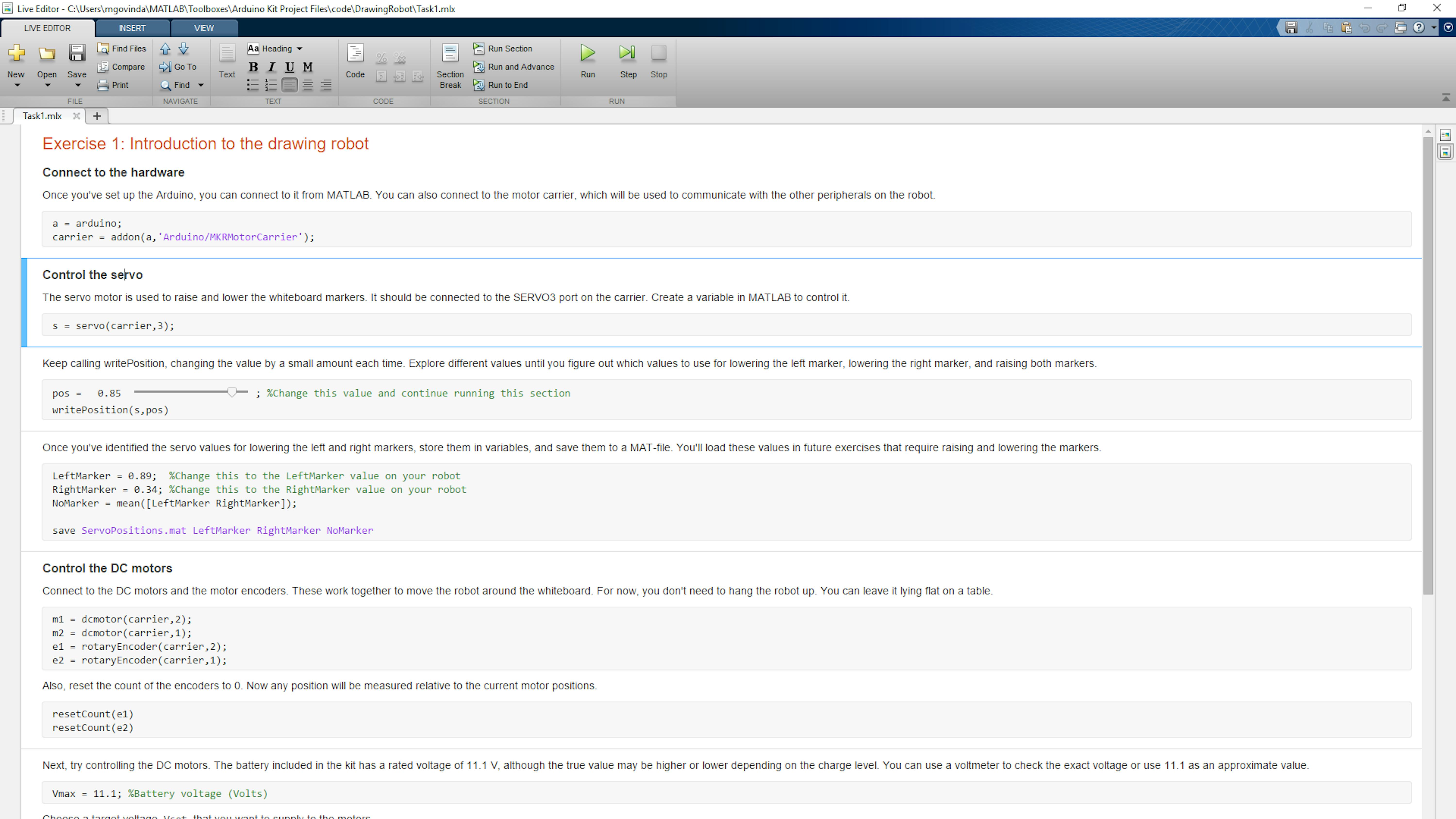
The following code section, contains a numeric slider control that defines the pos variable. Whenever you change the value of the slider, this section of code will execute, commanding the servo to move to a new position. In order to figure out the limitations for the position, you will have to change the value of pos in small increments until you find the servo position corresponding to one of the markers being fully lowered. Record that value and then repeat the process for the other marker. Because the robot, uses only one servo motor to control both markers, you simply need to change pos incrementally in the other direction until you find the servo position for lowering that marker. If you assembled the robot according to the assembly instructions, the left marker should be lowered at a servo position around 0.6 and the right marker should be lowered at a position around 0. After recording these values, you should also verify that a value of pos midway between these two extremes will have both markers up. In this way, you will have a single physical driver, the servo motor, to control three different states of the drawing mechanism: no markers drawing, marker 1 drawing, or marker 2 drawing.
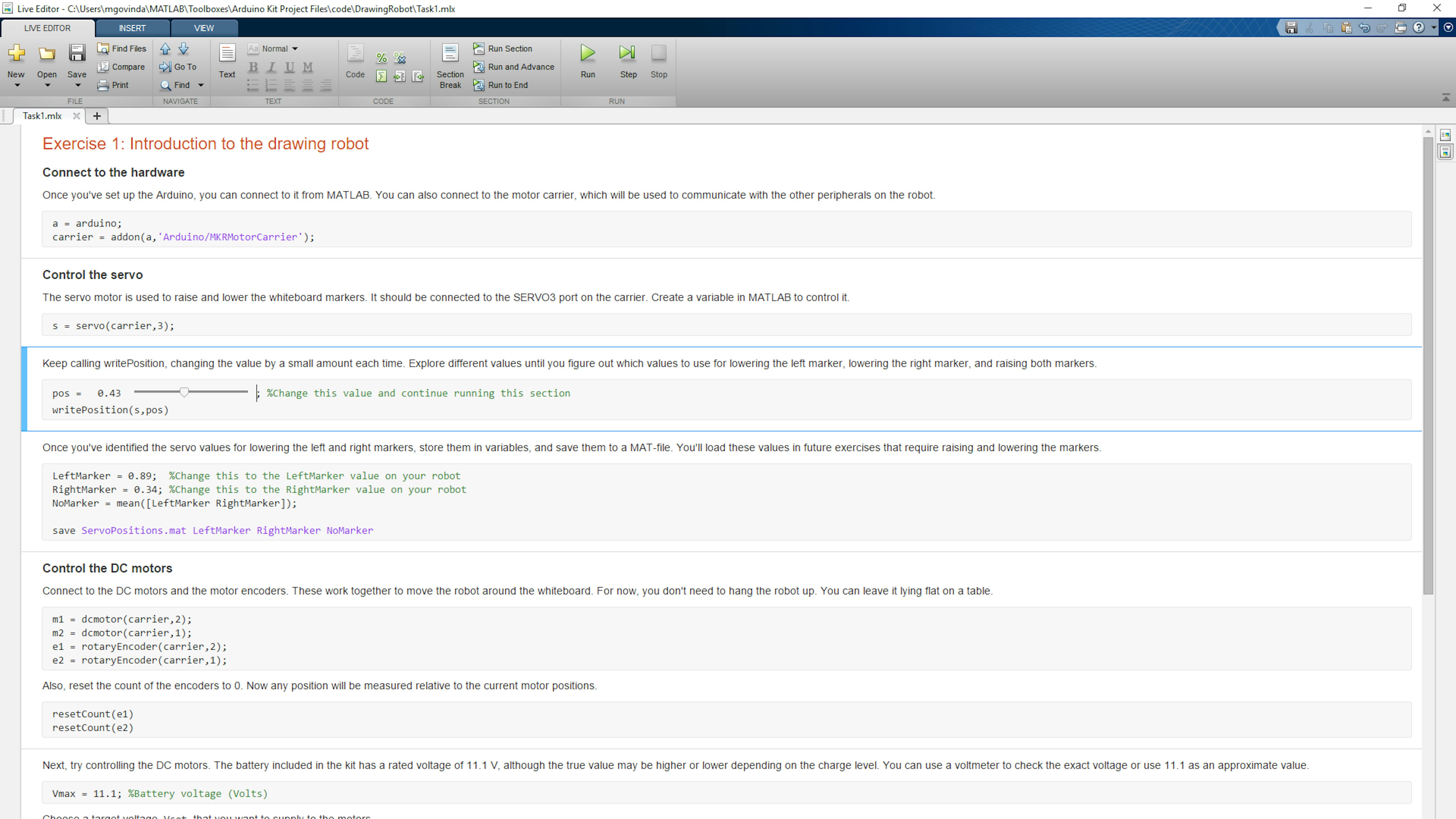
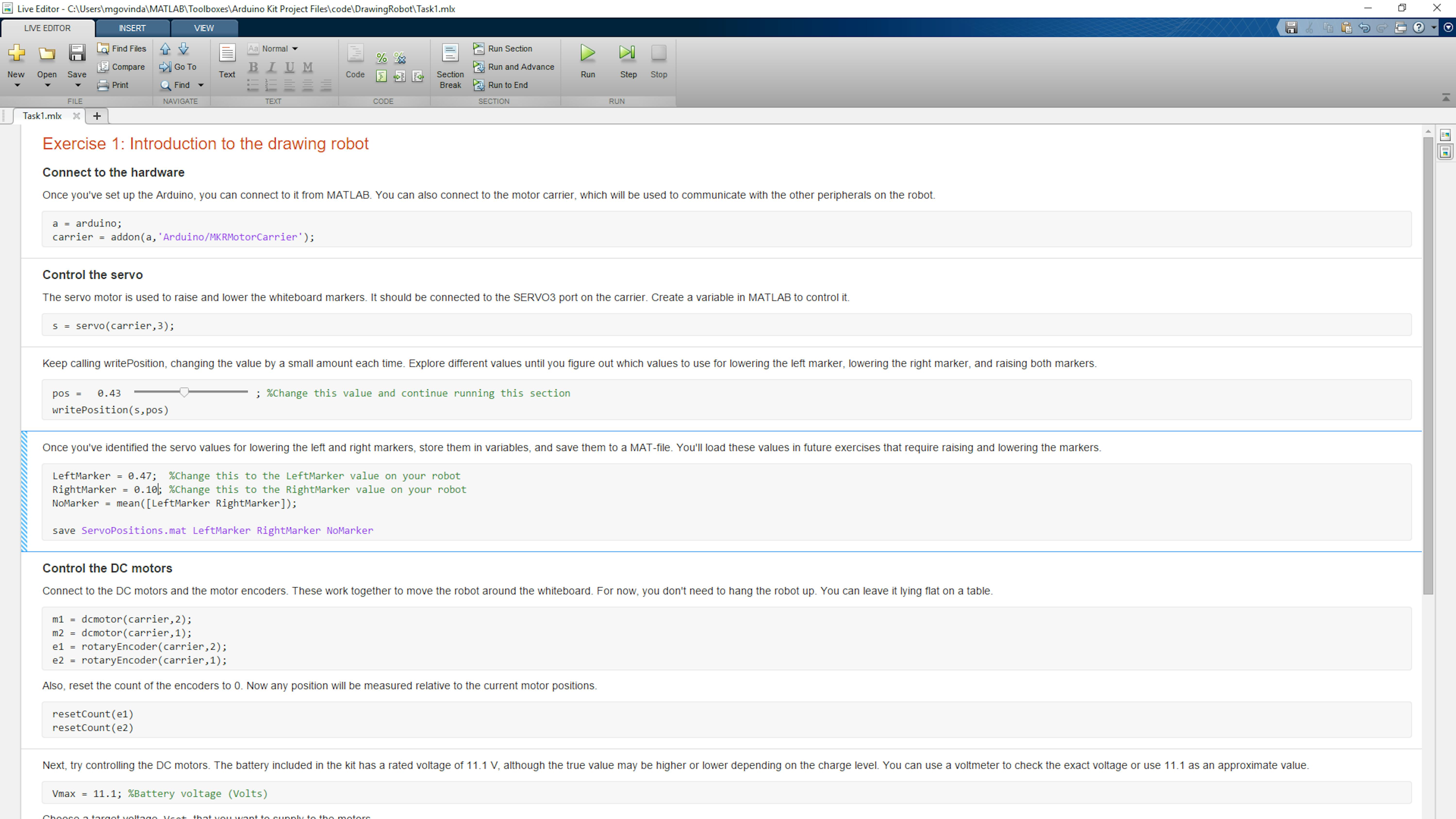
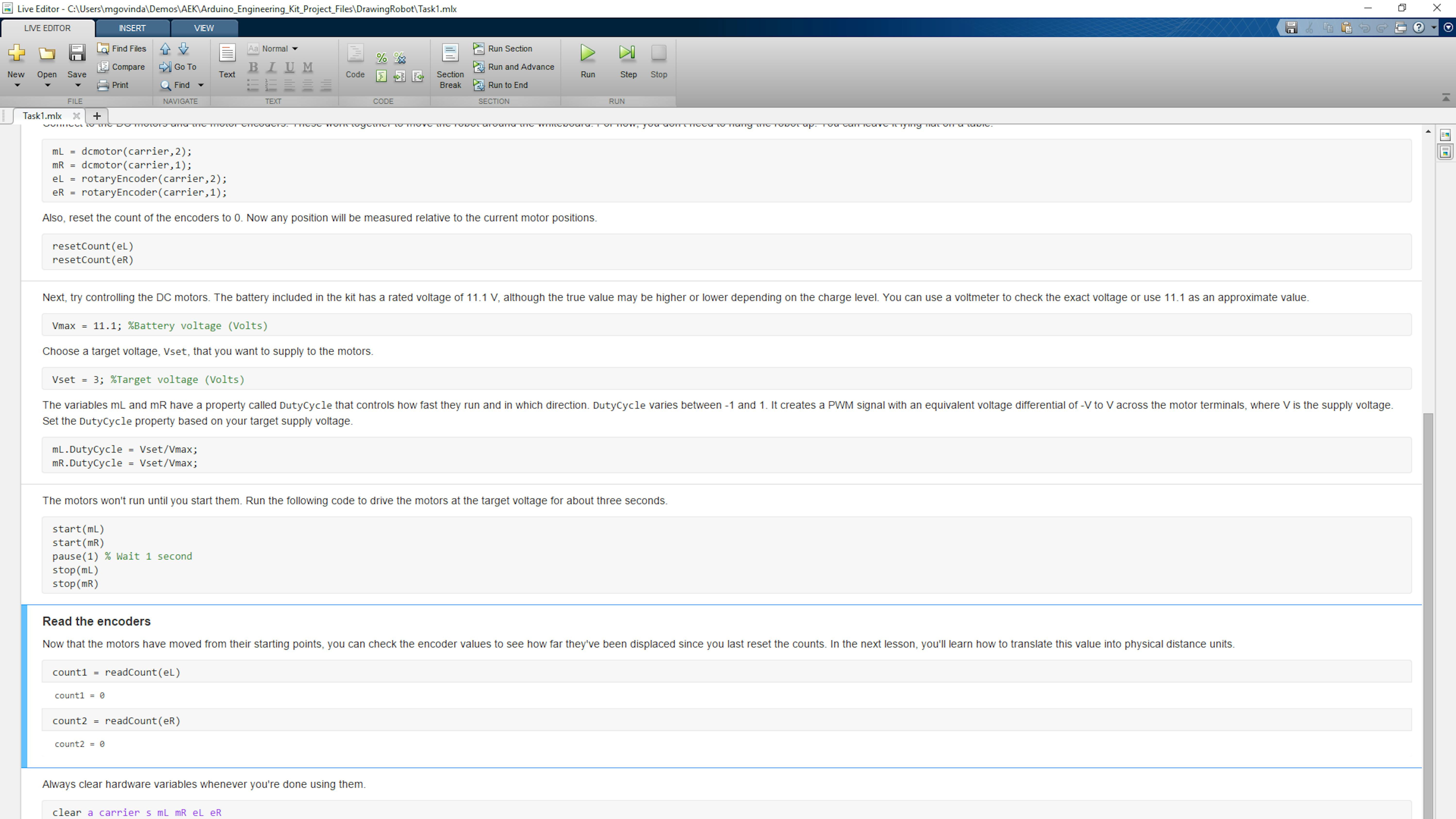
In the final code section under the heading Control the servo, enter your experimentally determined values for the servo position when lowering the left marker and the right marker. See the following screenshot for which values to update. Run this section of code to save these values to a MAT-file so you can load them for use in future exercises.
CONTROL THE DC MOTORS
Once you have controlled the markers, the next step is to figure out how to control the two DC motors that make the drawing robot move over the whiteboard.
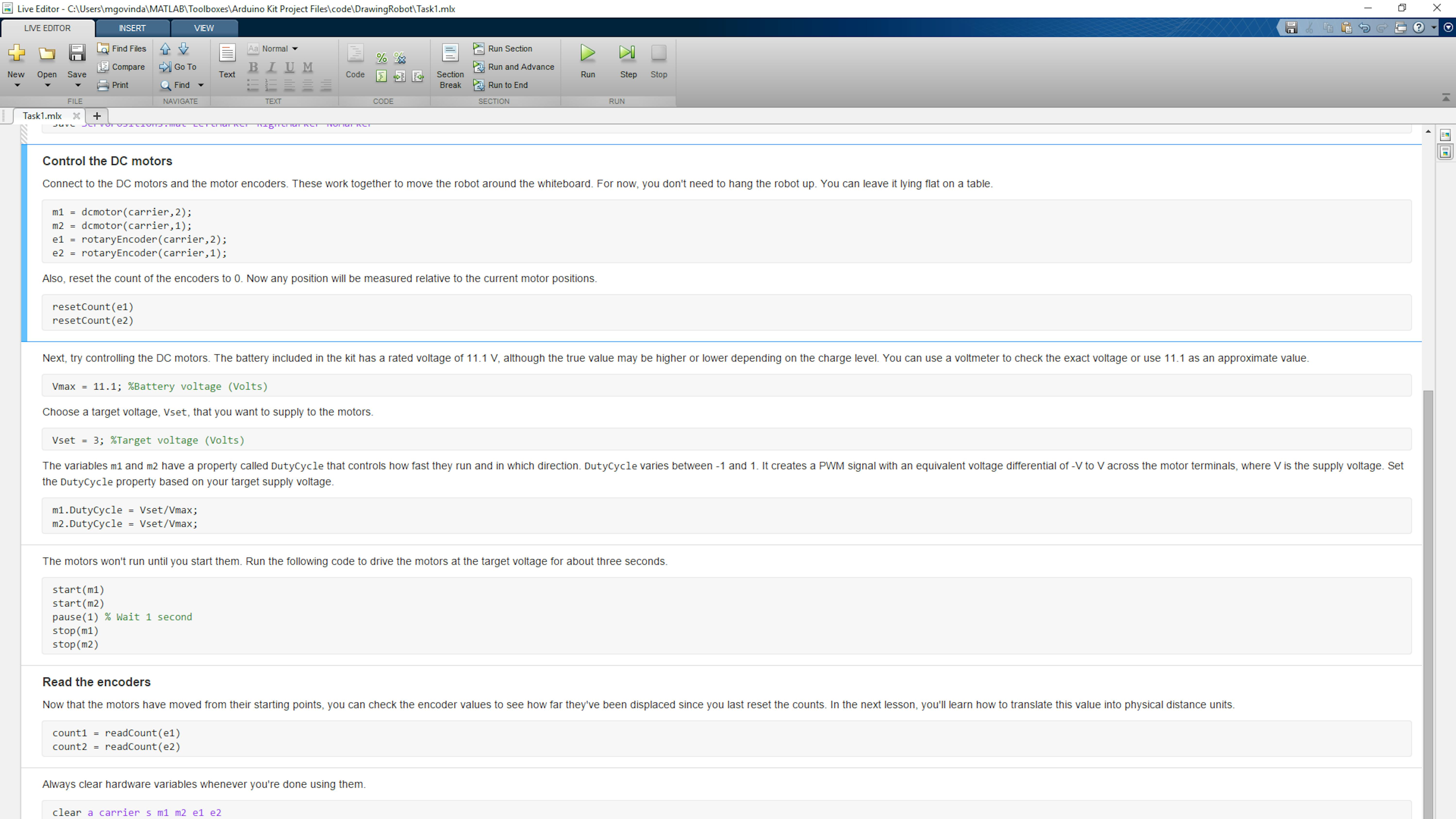
In this test, you will connect MATLAB to the motors and the motor encoders, specify a voltage to supply to the motors, and run the motors for about three seconds. First, identify and read the sections of Task1.mlx under the heading Control the DC motors. In this code,Vset is a target voltage to supply to the motor, and Vmax is the battery voltage. These parameters are used to compute a Speed value for the motors between 0 and 1, where 1 is maximum speed and 0 supplies no voltage to the motor. Run each of the sections of the live script under the heading Control the DC motors.
READ THE ENCODERS
As you know by now, DC motors require external control mechanisms to ensure that they are behaving as expected. In this case, we will use rotary encoders to measure the angle and speed of the motors while operating. After displacing the motors from their initial positions, you can read the count value from the encoders to determine how far each motor has turned in units of encoder counts. The conversion from counts to physical distances will be calculated in a later exercise. Run the code in the Read the encoders section of the live script Task1.mlx.
FILES
- Task1.mlx
LEARN BY DOING
Create a new MATLAB script. Write a series of commands that will run the left motor for three seconds, then stop and run the right motor for three seconds, then run the left motor in reverse for three seconds, then run the right motor in reverse for three seconds, and finally stop the motors. Run your script and check that it performs as expected. Read the counts from each of the encoders. How close are the motors to their starting positions? What might account for the difference? Reset the encoder counts and run the script again to see how consistent this result is.
Hang the robot up on the whiteboard. Run the left motor forward with a voltage of 4 Volts for 2 seconds. Run it in reverse with a voltage of -4 Volts for 2 seconds. How far did it move each time? In which direction did it move faster? Why? How is the behavior different from when you have the robot flat on the table?
EXERCISE 2:
4.2 Whiteboard coordinate system
In this exercise, you will define distances that describe the position of the robot on the whiteboard. You will hang the robot up on the whiteboard and move it around using an app. Then you will compute the new position of the robot in x-y coordinates based on encoder measurements.
In this exercise, you will learn to:
- Use built-in UI functions to get user input
- Apply geometry concepts to code
- Use MATLAB apps
- Write MATLAB functions
DEFINE DISTANCES ON THE WHITEBOARD
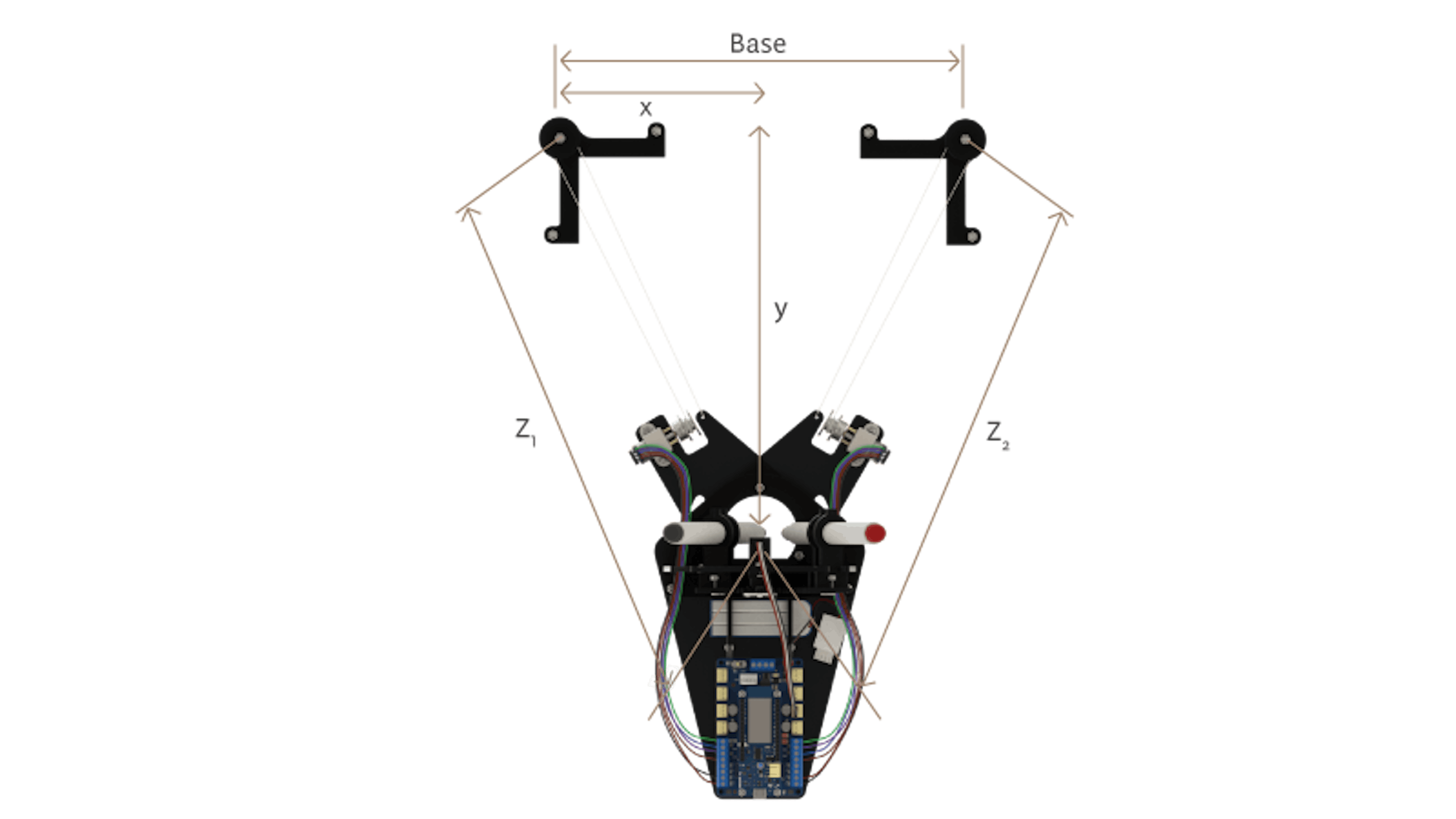
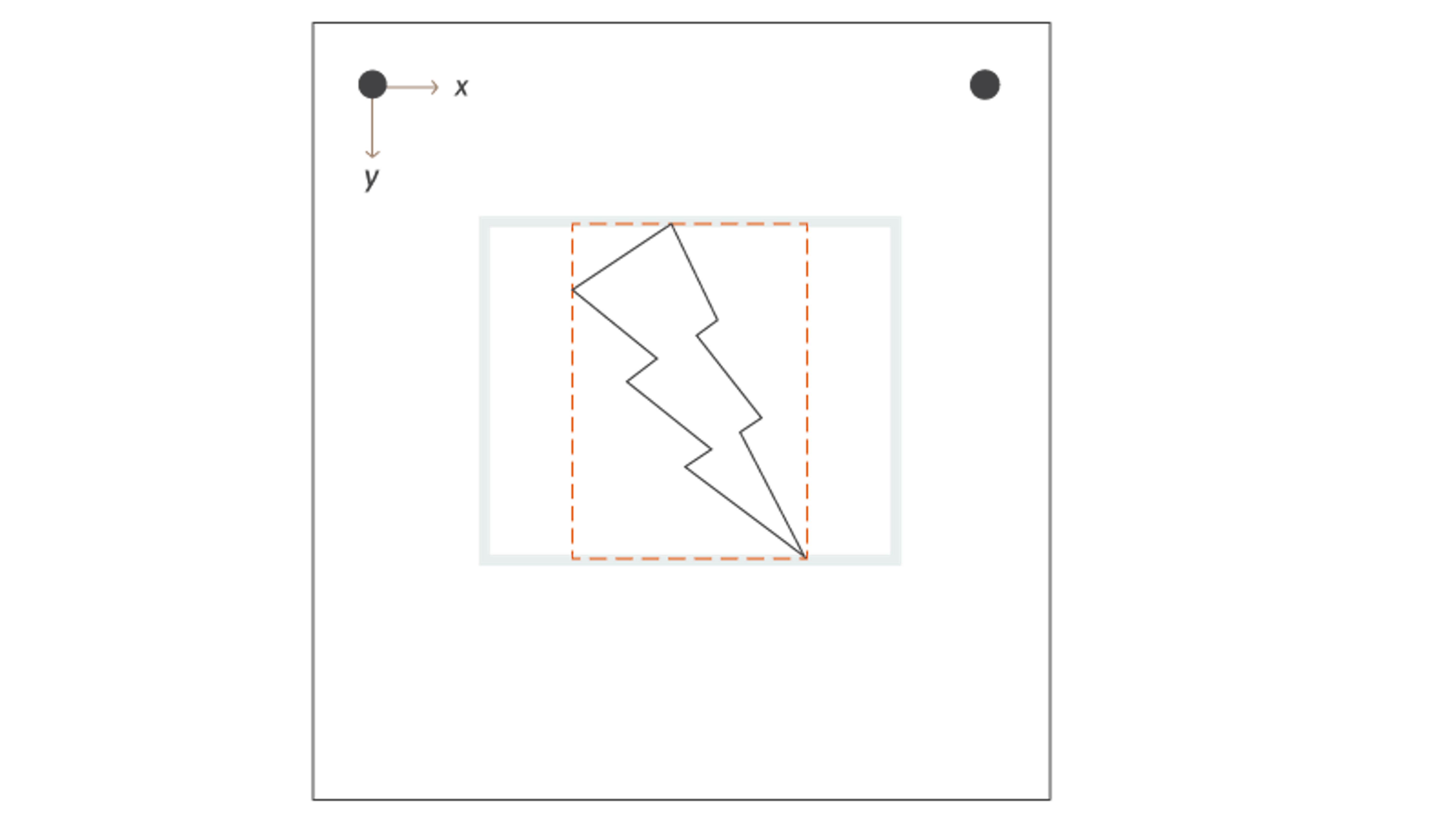
Imagine hanging the robot up on the whiteboard. Define the values y, Base, Z1, and Z2 as shown in the following diagram. The black circles at both sides of the diagram represent the pulleys from which you hang the robot, while the robot is in the center of the image, hanging from two strings connected to the robot arms, where the motors are located. Note how the strings go from the robot arm to the pulley and come back to the motor. Also observe that x and y positions on the whiteboard are measured with respect to the left-most pulley, with x being the horizontal distance to the right of the pulley and y being the vertical distance down from the pulley.
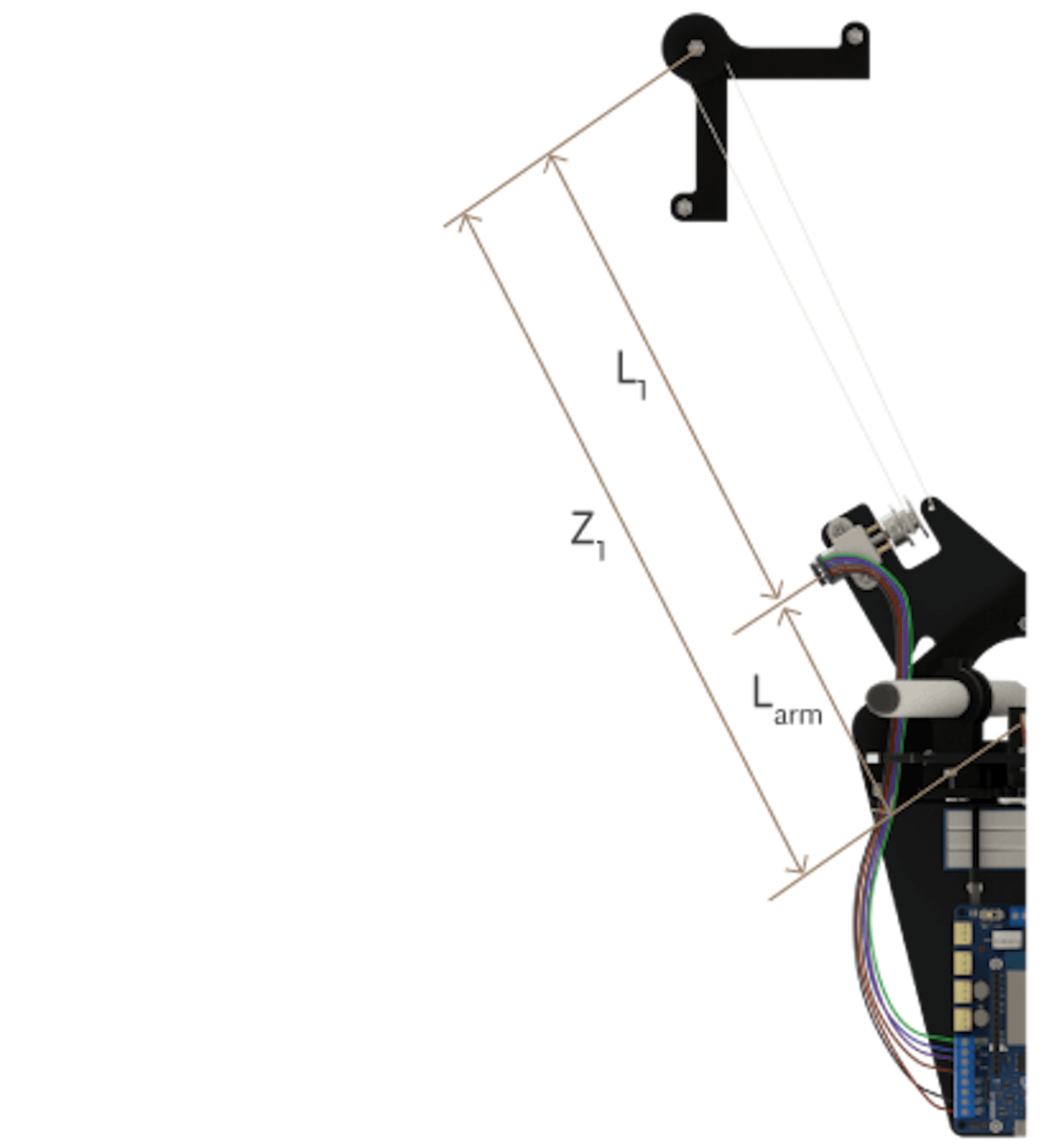
We can divide ${ Z1}$ into the motor arm $L_{\text{arm}}$ and then length from the string from the motor to the pulley (${ L1}$). We'll do the same for ${ Z2}$ with $L_{\text{arm}}$ and ${ L2}$.
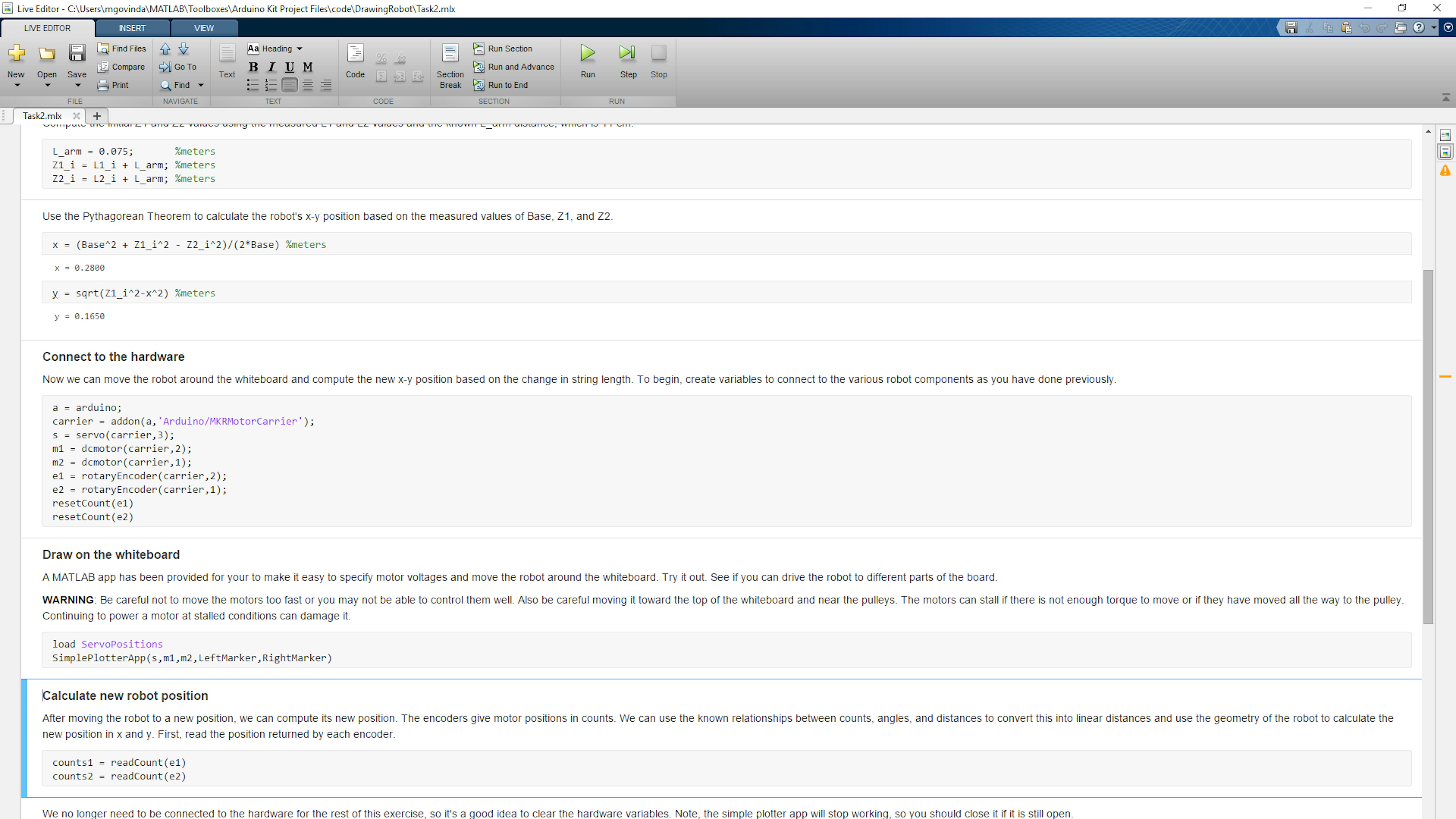
APPLY THE PYTHAGOREAN THEOREM TO COMPUTE POSITION
Before we start moving the robot, we need to measure ${ Base}$,${ L1}$ and ${ L2}$. We will use a known value of $L_{\text{arm}}$ to compute ${ Z1}$ and ${ Z2}$. As the robot moves around the whiteboard, we'll update ${ Z1}$ and ${ Z2}$ based on the encoder measurements. To get the values of x and y, we can use these known values of ${ Z1}$ , ${ Z2}$ and ${ Base}$ along with the Pythagorean Theorem. If you drop a perpendicular line from the marker to the line between the two pulleys, two right triangles are formed, as shown in the following diagram.

The sides of these triangles have the following relationships.
$Z_1^2=x^2+y^2$
$Z_2^2=({Base}-x)^2+y^2$
If we solve the second equation for ${ y^2}$, the first equation can be rewritten as
$Z_1^2=x^2+[Z_2^2-({Base}-x)^2]$
Expanding this equation and solving for x, we end up with the following equations to solve for x and y sequentially.
$x=\frac{{Base}^2+Z_1^2-Z_2^2}{2\ast {Base}}$
$y=\sqrt{Z_1^2-x^2}$
UNDERSTAND INPUT DIALOGS
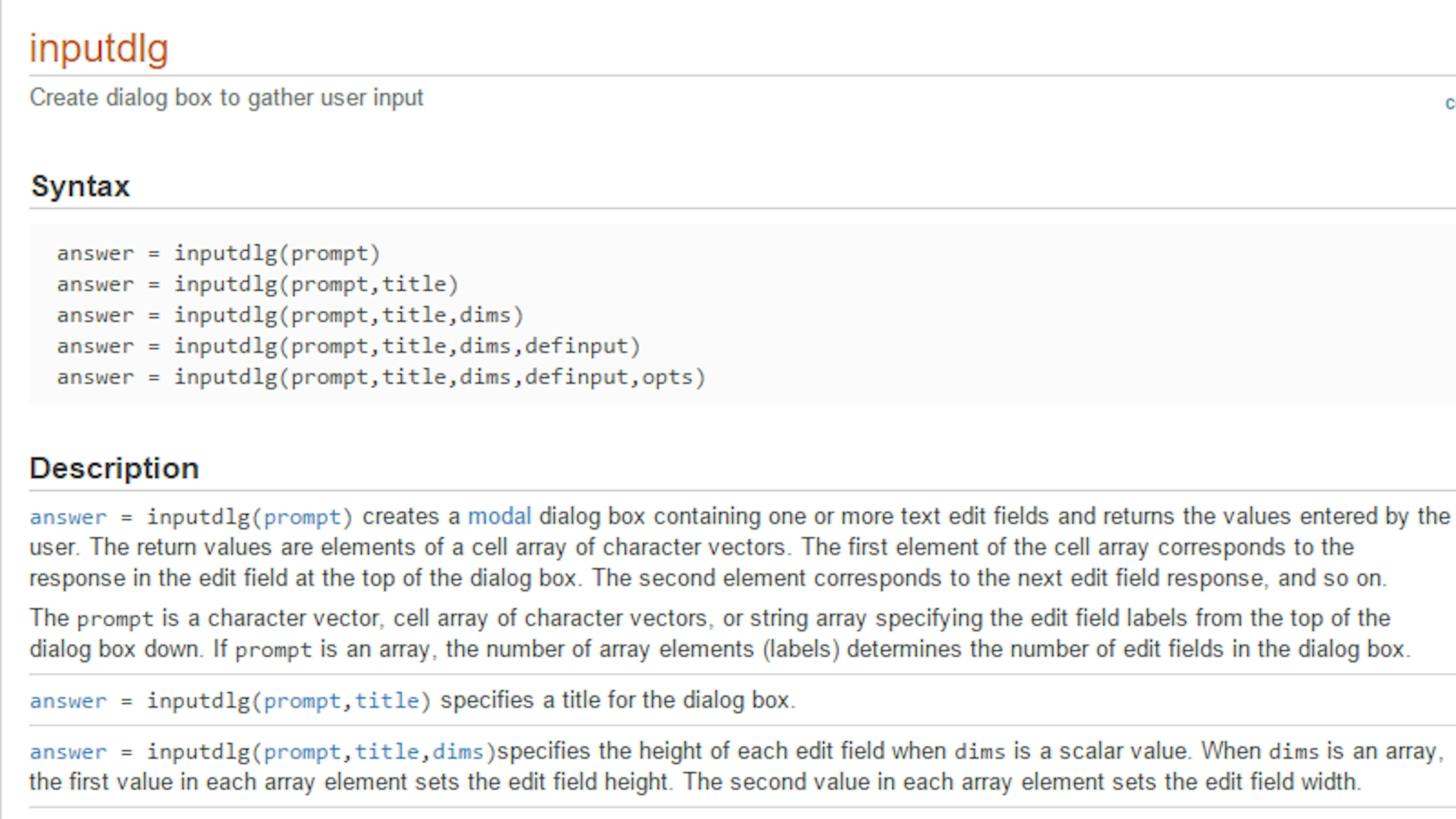
An easy way to allow a user to interact with your MATLAB program is with a dialog box. Dialog boxes are simple apps that can report messages, gather input, or allow the user to interact with the file system. See the MATLAB documentation on Dialog Boxes for a list of dialog boxes available in MATLAB.To request input from a user, use an input dialog. This can be created with the inputdlg function. There are several options for configuring this dialog box, so you should review the documentation page to better understand the available syntax. Open the documentation page directly from the MATLAB command prompt by typing the following:
>> doc inputdlg
Read the Syntax and Description sections of this documentation page to understand all the allowed input arguments for this function.
Then scroll down to the Examples section. One of the advantages of opening the documentation from within MATLAB rather than online is that you can run examples directly from the documentation page. Highlight the code from Example 1, then right-click and select Evaluate Selection.
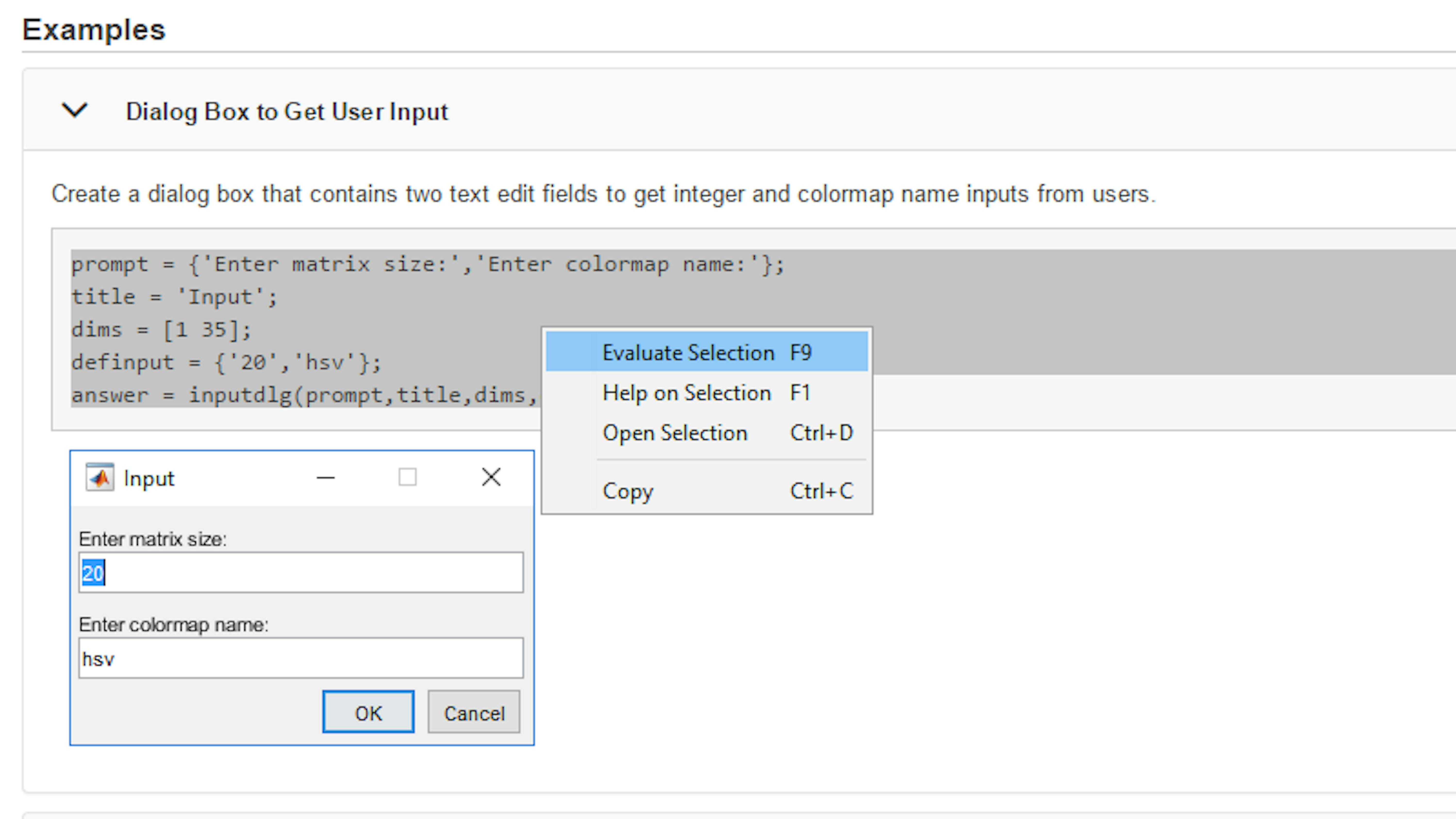
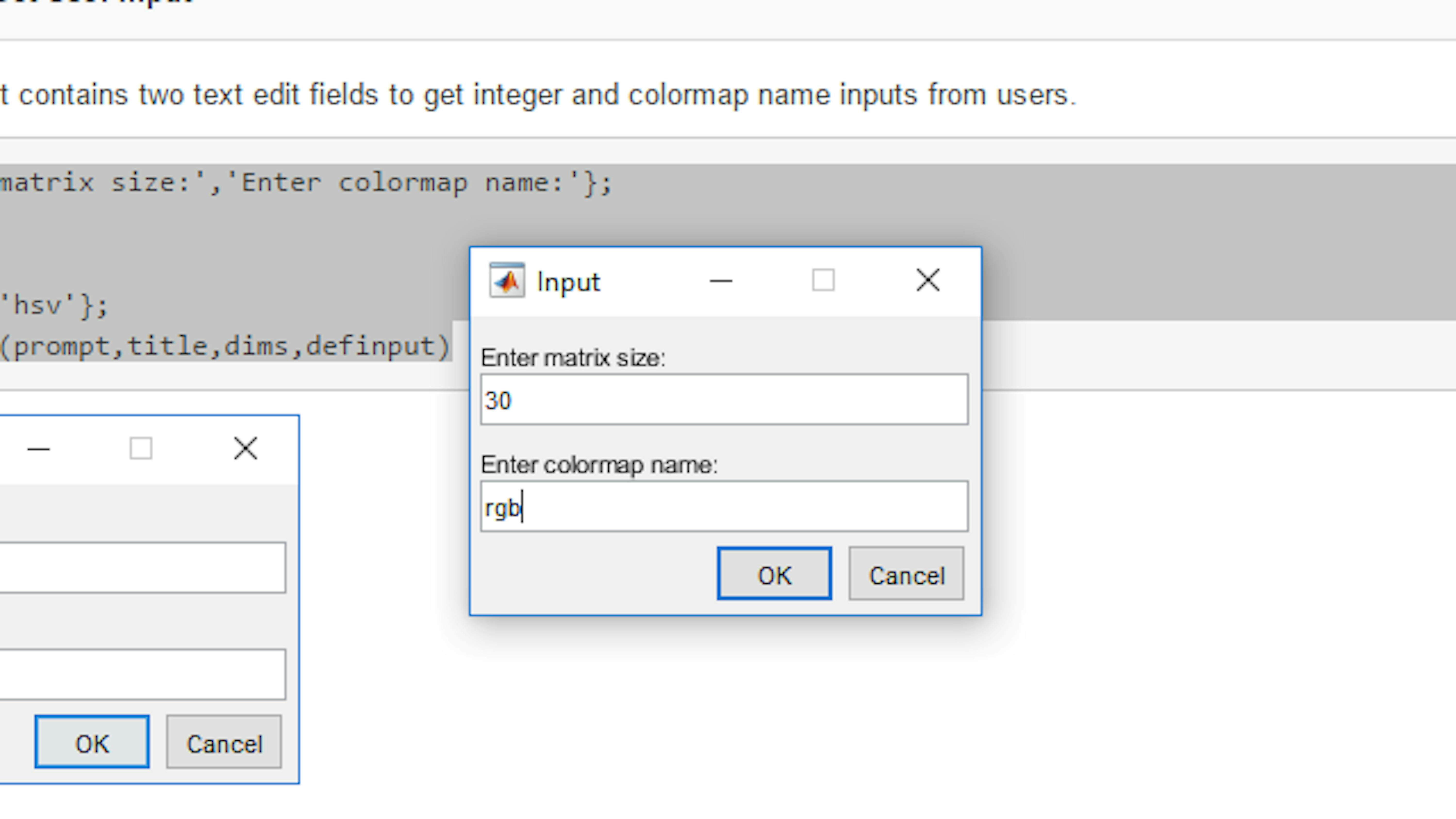
When the dialog launches, enter new values for matrix size and colormap name. Click OK.
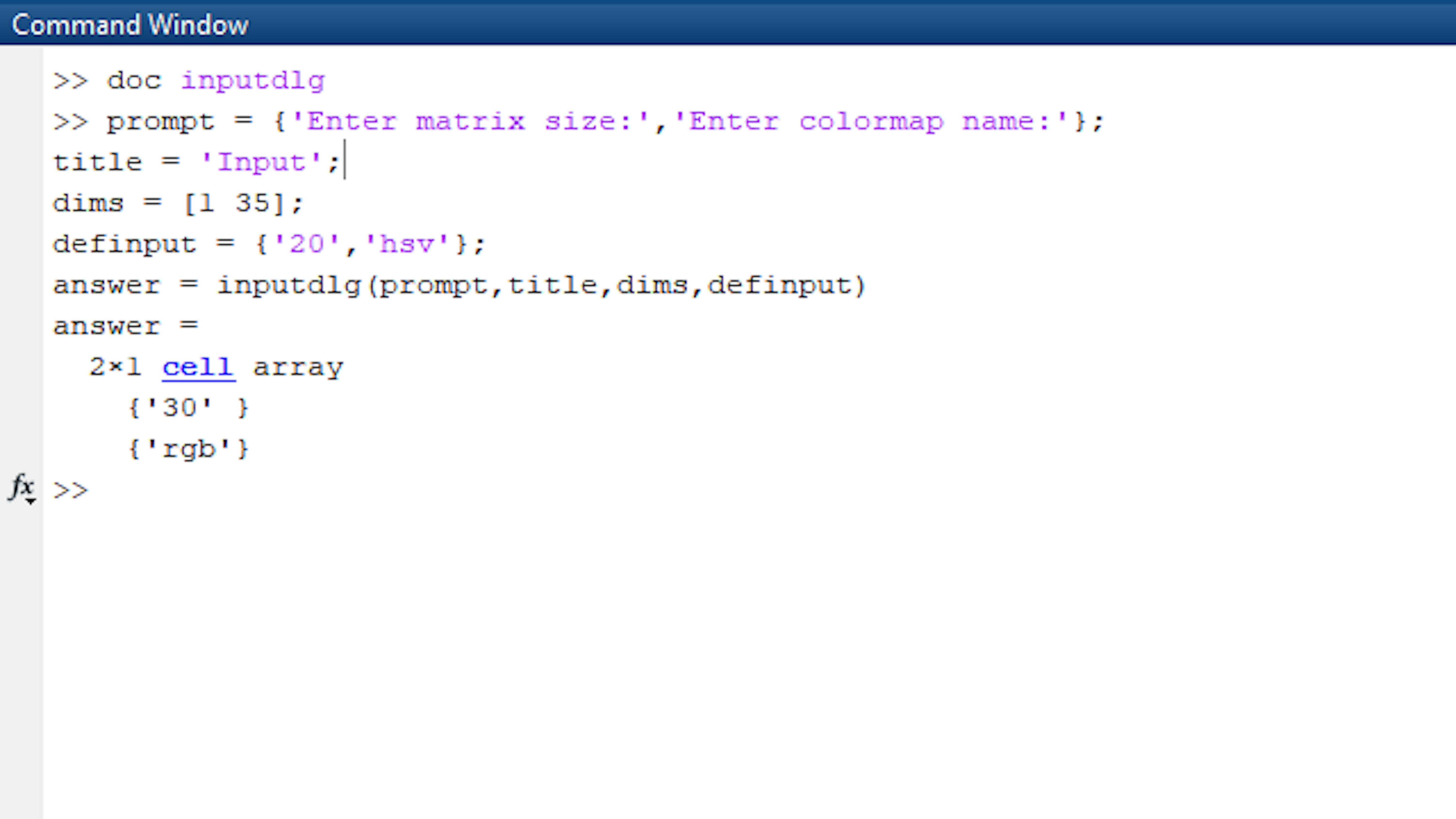
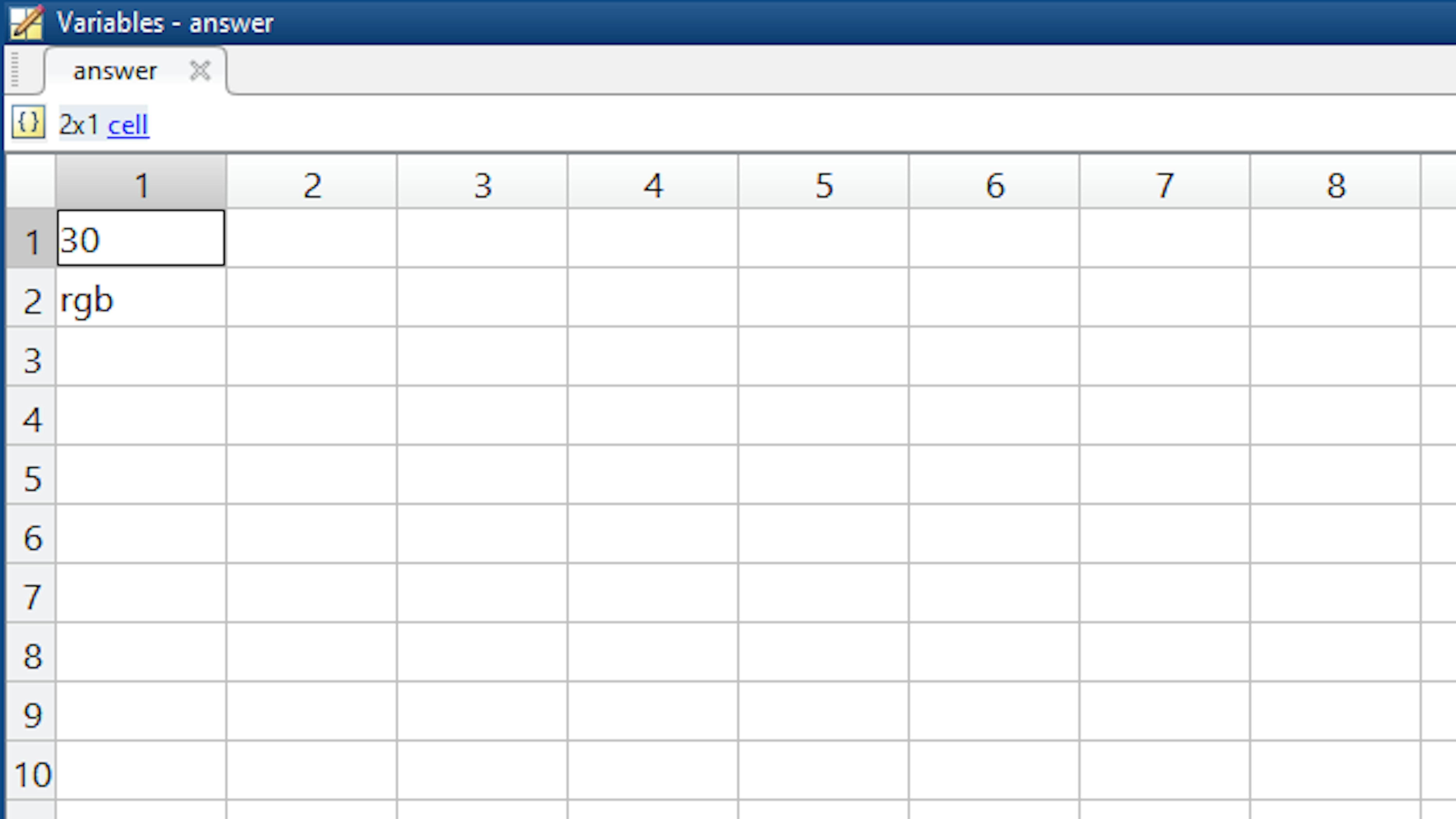
Return to the MATLAB Command Window. Note that the example code you evaluated appears here and in your Command History. Also, note there is a new answer variable in the Workspace. Check its value.
Now try running the code from other examples or write your own code that creates a dialog to request input from a user. In the next section, you'll use an input dialog to update the robot measurements without having to edit your code each time you run it.
FIND A STARTING POSITION
Open the live script Task2.mlx by typing in the Command Window:
>> edit task2
Measure the Base , L1 , and L2 distances on your robot with a meterstick, ruler, or tape measure. Then follow the instructions of the first four sections of Task2.mlx under the heading Find starting position, entering these values where appropriate. Please note that all measurements should be written in meters. This will allow you to calculate the starting x-y position of the robot on the whiteboard.
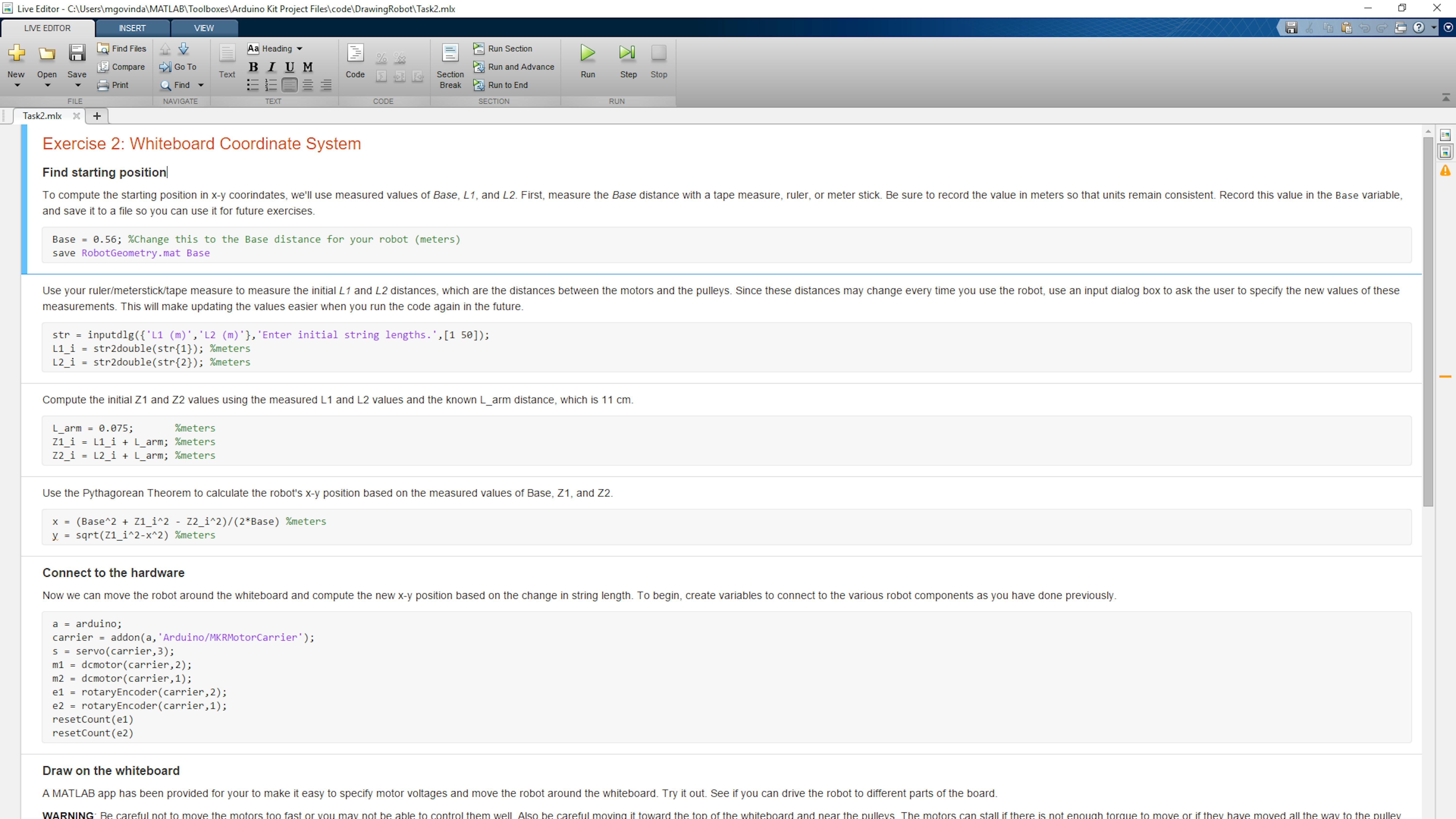
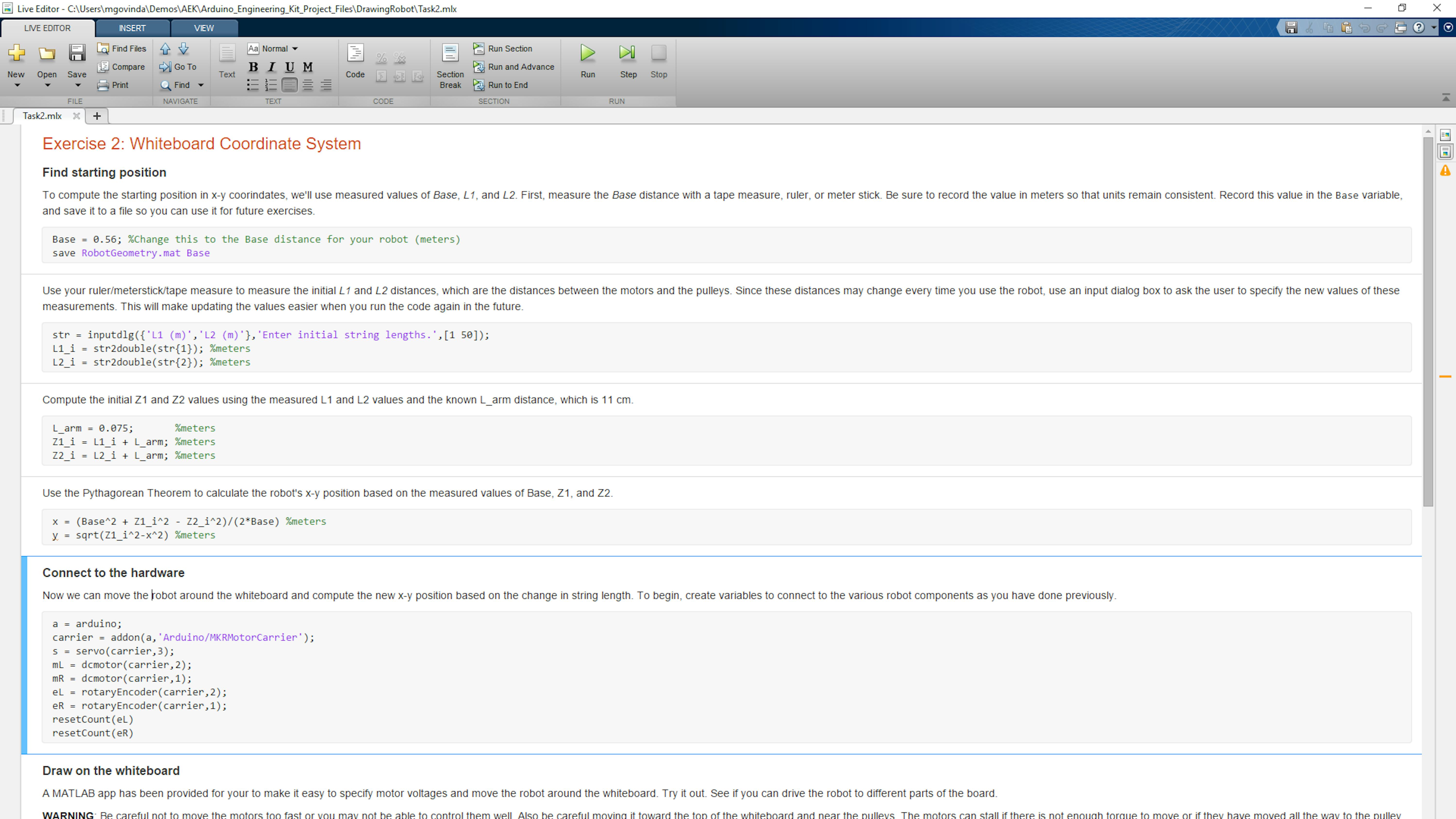
CONNECT TO THE HARDWARE AND DRAW ON THE WHITEBOARD
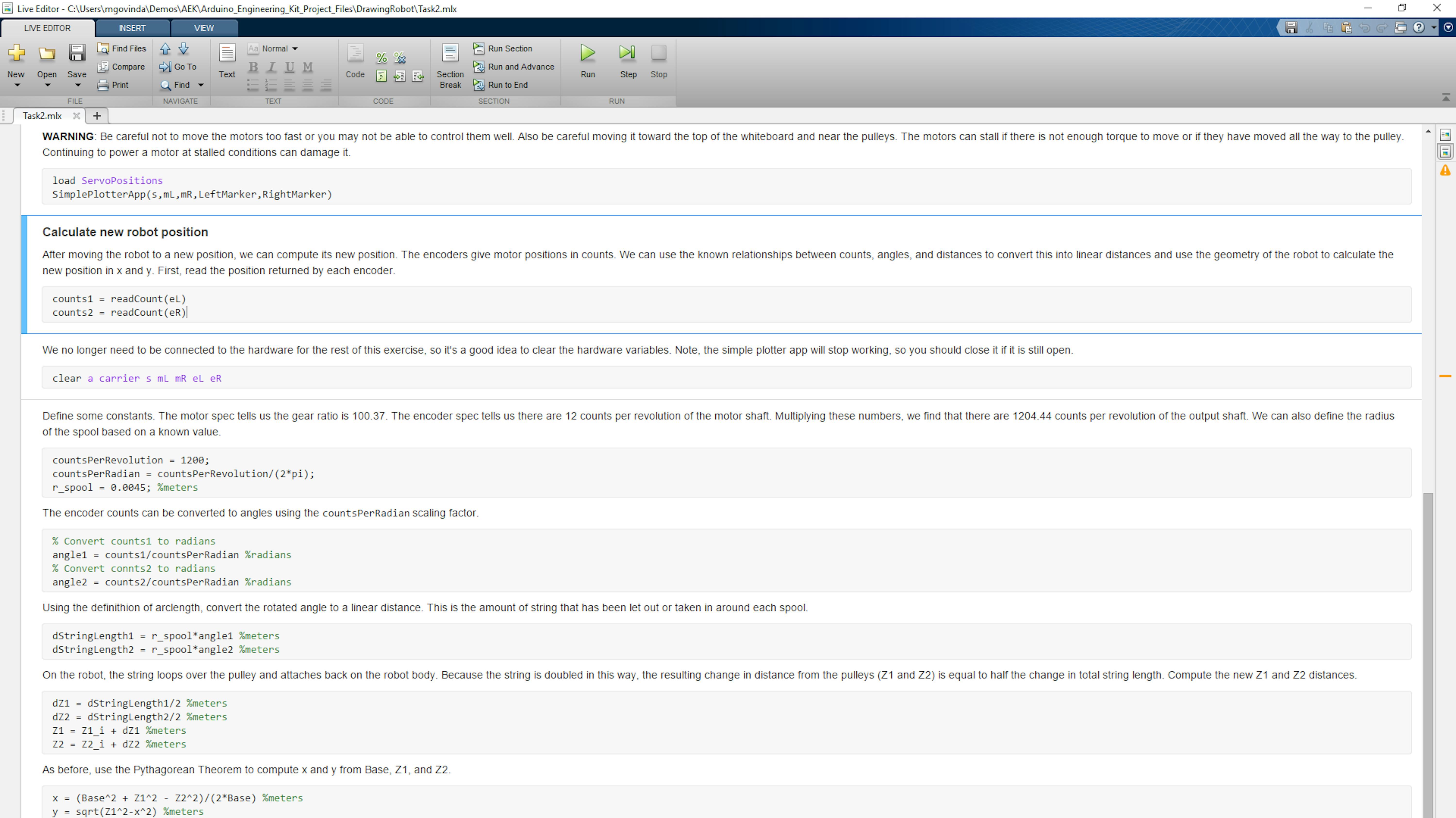
As you did in the previous exercise, you will now connect to the Arduino and control the motors. This time, however, you will use an interactive application (or app ) in MATLAB to start and stop the motors and specify their voltages. MATLAB apps typically have a graphical user interface and code to perform a specific task. The drawing robot project provides an app called SimplePlotterApp that can be used to interactively control the robot's motors. Run the code in the Connect to the hardware and Draw on the whiteboard sections in the live script Task2.mlx. This will launch an app with buttons allowing you to interactively start and stop each of the motors and change their speed. Be careful not to move the motors too fast or to pull the robot all the way up to the top of the whiteboard where the motors may stall.
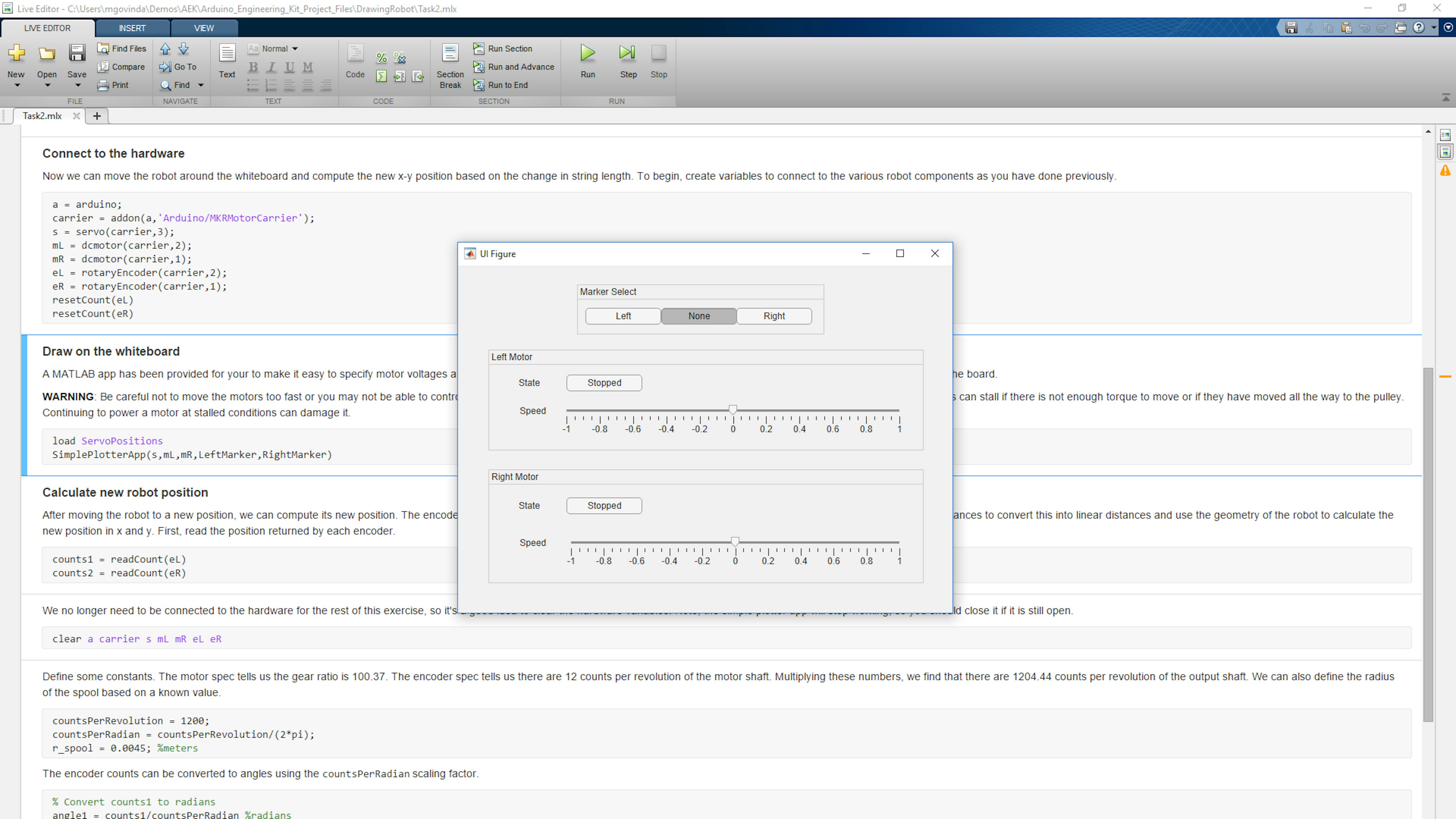
COMPUTE THE NEW ROBOT POSITION
With the information you have so far, it is now possible to compute the new position of the robot on the whiteboard in x-y coordinates. You can now read the new encoder counts, convert these values to angles, and then convert these angles to distances. Finally, you can use the robot geometry to convert the distances into an x-y position on the whiteboard. To start, read the current count value for the two encoders. You can then clear the hardware variables in MATLAB, since you'll no longer need them for this exercise. Run the first two sections of Task2.mlx under the heading Calculate new robot position. Then run these sections.
You have the motor positions in units of counts. How do you convert this to an x-y position? First, you can convert the position in counts to an angular position. You know the number of counts per revolution from the motor spec sheet. The angular position of the motor is therefore computed as follows:
$C_{{rad}}\frac{{counts}}{{rad}}=\left(1204.44\frac{{counts}}{{rev}}\right){\cdot}\left(\frac{{rev}}{2\pi {rad}}\right)$
$\theta =\frac{C{counts}}{C_{{rad}}\frac{{counts}}{{rad}}}$
The amount of string spooled or unspooled by the motors is related to the angle it has rotated through and the radius of the spool. In fact, we can calculate it using the definition of arclength.
${\Delta}{StringLength}=r_{{spool}}\cdot\theta$
On the robot, the string loops over the pulley and back to the robot body. Because the string is doubled, the resulting change in distance from the pulleys (Z1 or Z2) is equal to half the change in total string length. We can compute the new Z lengths based on this relationship.
${\Delta}Z=\frac{{\Delta}{StringLength}} 2$
$Z={\Delta}Z+Z_i$
The new robot position is fully defined by the Base, Z1, and Z2 lengths. As we did earlier in this exercise, we can use these values to compute the current values of x and y.
$x=\frac{{Base}^2+Z_1^2-Z_2^2}{2\ast {Base}}$
$y=\sqrt{Z_1^2-x^2}$
To perform these calculations in code, run the remaining sections of Task2.mlx under the heading Calculate new robot position.
ENCAPSULATE CODE IN FUNCTIONS
We'll want to repeat some of the tasks performed in this exercise again in the future. To better organize our code, reduce repetition, and make it easy to solve these problems in the future, we can create MATLAB functions that perform specific tasks.
First write a MATLAB function for requesting the initial string length measurements from the user. In the MATLAB Desktop, select New>Script . This will create an empty MATLAB file. Enter the following code and save the file as initialPosition.m.
function Z_i = initialPosition()
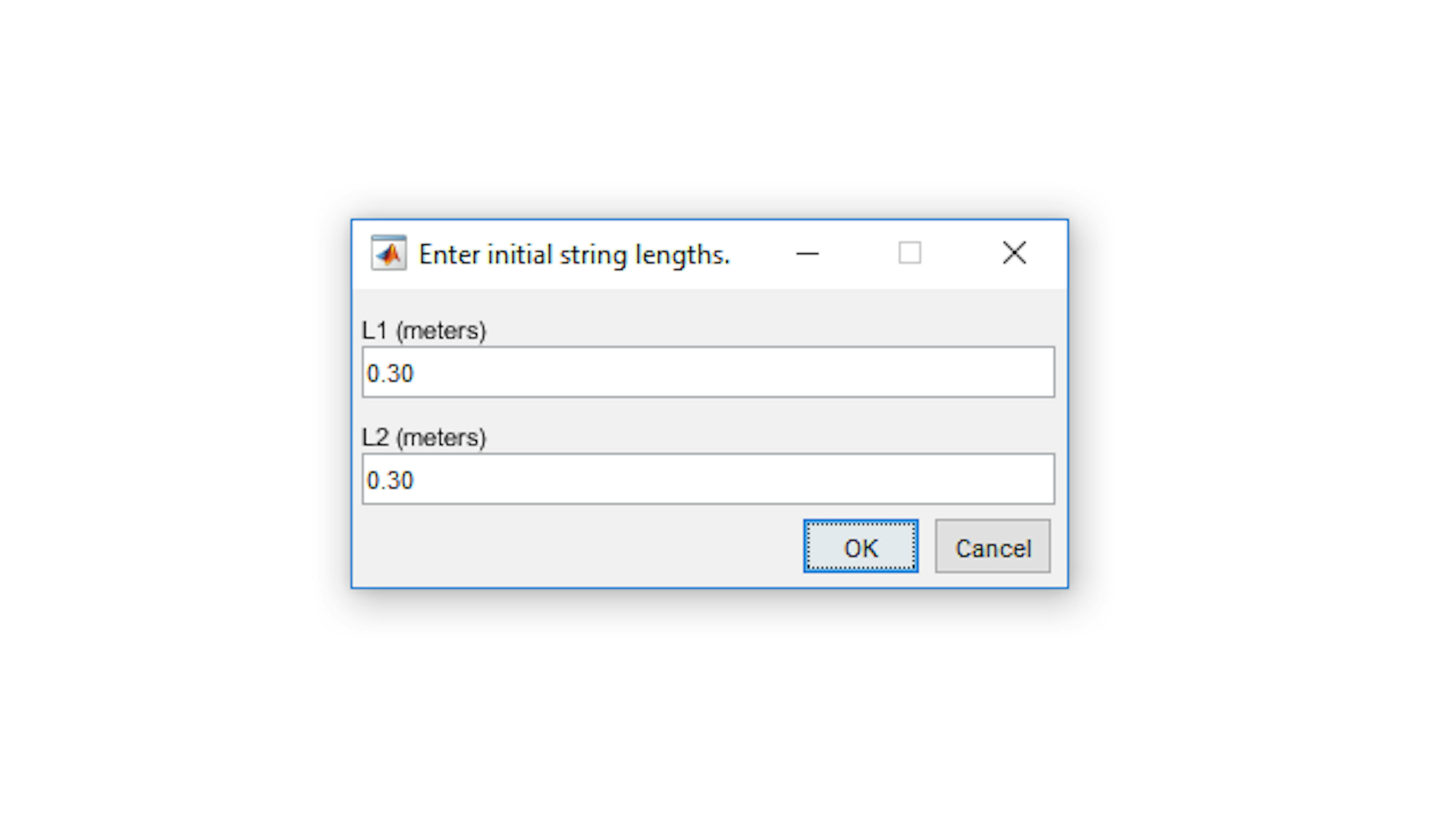
str = inputdlg({'L1 (meters)','L2 (meters)'},'Enter initial string lengths.',[1 50]);
L1_i = str2double(str{1}); %meters
L2_i = str2double(str{2}); %meters
L_arm = 0.075; %meters Z_i = [L1_i L2_i] + L_arm; %metersTry it out. Call your new function from the MATLAB Command Window, enter the string length values, click OK, and observe the result.
>> Z_i = initialPosition
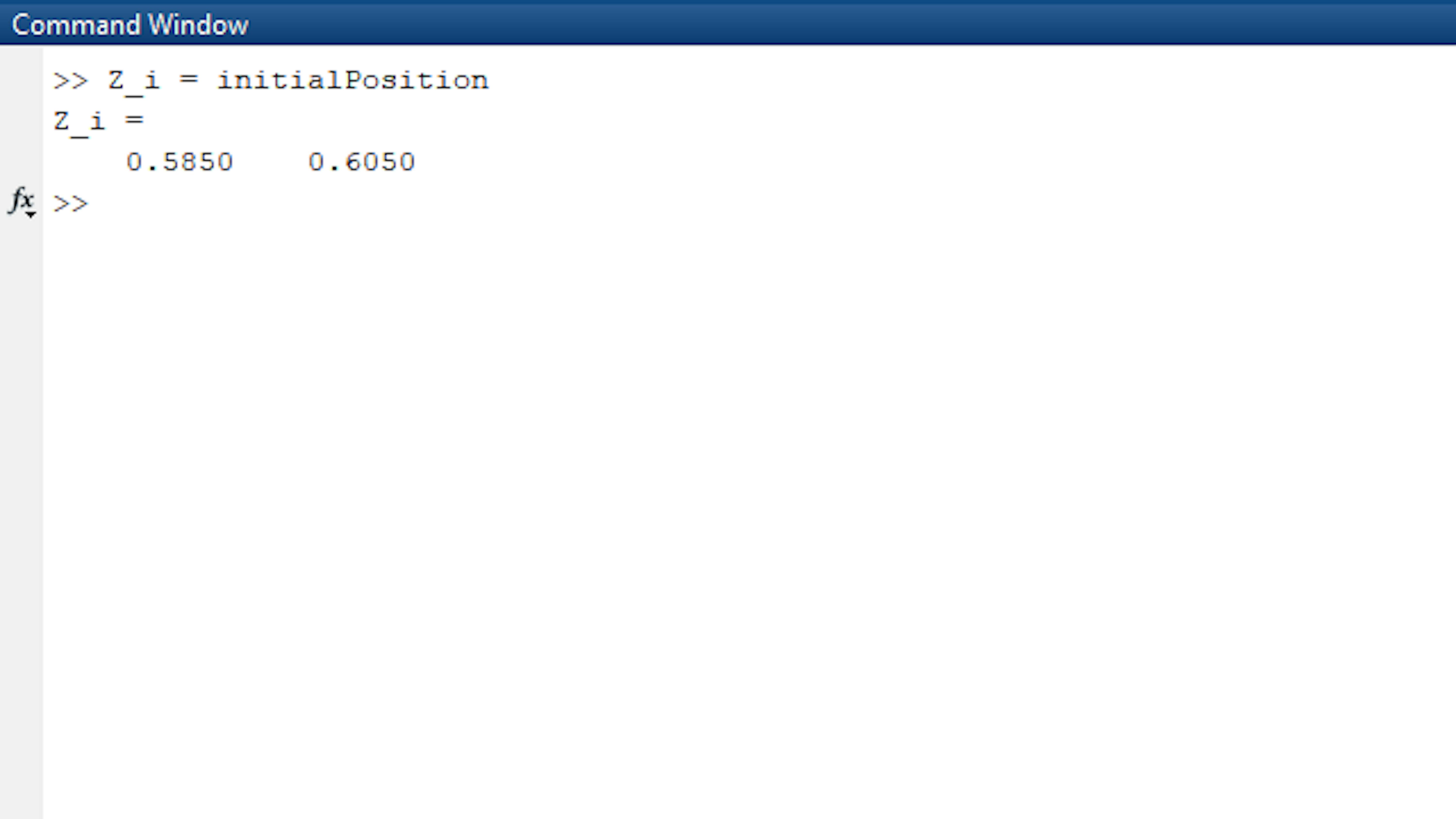
Note that we’re now using a single variable Z_i to contain both Z1_i and Z2_i. This variable has size 1x2 and can be indexed with the syntax Z_i(1) and Z_i(2) to extract its components. Let’s also put ourcounts1 and counts2 variables together into a single variable counts. This will make our code much simpler. Run the following line at the MATLAB Command prompt to create the counts variable.
>> counts = [counts1 counts2]
Next, write a function for converting the measured encoder counts to an x-y position on the whiteboard. Create a new function called countsToXY.m and include the following code
funcfunction xy = countsToXY(counts,Z_i,Base) % Define constants
countsPerdRadian = countsPerRevolution/(2\*pi);
r_spool = 0.0045; % Convert counts to angle
phi = counts/countsPerRadian; % Convert angle to change in string length
dStringLength = r_spool\*phi; % Convert change in string length to change in Z
dZ = dStringLength/2; %Add change in Z to initial Z to get current Z
z = z_i + dz; % Compute x and y from Z1 and Z2
x = (Base^2 + z(1)^2 - z(2)^2)/(2\*Base);
y= sqrt(z(1)^2-x^2); xy = [x y];
end
Verify that this function behaves correctly. You should still have the variables counts , Z_i , and Base in your workspace. Run the following at the command prompt, and check that the x-y position is correct.
>> xy = countsToXY(counts,Z_i,Base)FILES
- Task2.mlx2
- countsToXY.m
- initialPosition.m
LEARN BY DOING
If you click Cancel instead of OK on the input dialog box, what happens? What happens when you continue running the code? Is this what you would expect? Describe the desired behavior and how you would design your code to behave this way when a user clicks the Cancel button. Using just the SimplePlotterApp app, try to control the robot and draw a shape. What shapes are easy to draw? What shapes are difficult?
Run an experiment to measure the radius of the spool. Reset the encoder. Then write a script that will spin the motor for a few seconds in a direction that unspools the string. Hold onto the string and don't let it slip off the edge of the spool. When the motor stops, measure (with a ruler) how much string was let out. Read the encoder count to see how far the motor turned and convert this value to an angle. Now use the equation for arclength to compute what the radius must be for a circle that unspooled that amount of thread and spun through that angle. Compare your experimentally determined radius to the radius provided in the exercise.
EXERCISE 3:
4.3 Move to specified points
In this exercise, you will choose specific locations on the whiteboard and move the robot to them. You will learn about more complex MATLAB functions, and you'll use these functions to control the robot. Finally, you'll have a short algorithm that can raise and lower the marker and draw simple shapes.
In this exercise, you will learn to:
- Construct simple MATLAB algorithms
- Write vectorized code
- Use nested flow control structures (for, while, break)
CHOOSE A POSITION TO MOVE TO
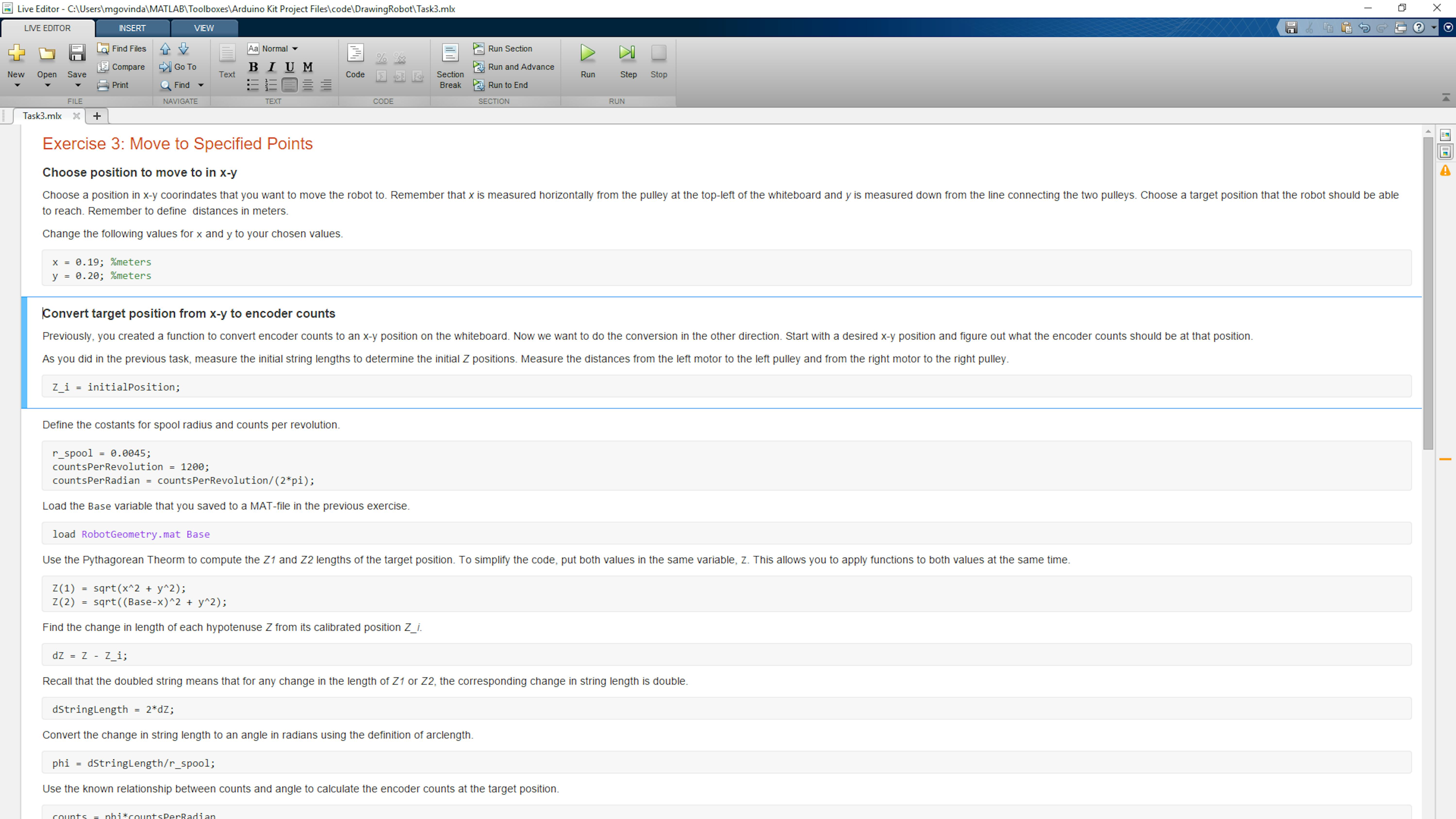
Let's move on with the next exercise. Hang the robot up on the whiteboard, making sure that both pulleys are located over the same horizontal line. Choose a target position on the whiteboard where you'd like to move the marker, and make sure it's a point that is reachable by the robot. Measure the x and y coordinates of that point using the whiteboard coordinate system where x is the horizontal distance to the right of the top-left pulley and y is the vertical distance down from the line connecting the pulleys. Open the live script Task3.mlx.
>> edit Task3
In the first section, called Choose position to move to in x-y, replace the values of x and y with the values for the point you want your robot to move to. Make sure that all measurements of the coordinates are in meters. Run this section.

CONVERT TARGET POSITION TO ENCODER COUNTS
Next, you will use the same relationships between counts, angles, and whiteboard distances that you used in the previous exercise. However, instead of taking measured counts and computing an x-y coordinate, you'll take a target x-y coordinate and compute the encoder counts for that position. To do this, use the same equations from the previous exercise, but reverse the order. Starting with the x-y coordinate, you can use the Pythagorean Theorem to calculate the Z1 and Z2 lengths.
$Z_1=\sqrt{x^2+y^2}$
$Z_2=\sqrt{\left({Base}-x\right)^2+y^2}$
Then you can compute the changes in Z and convert that to a change in string length.
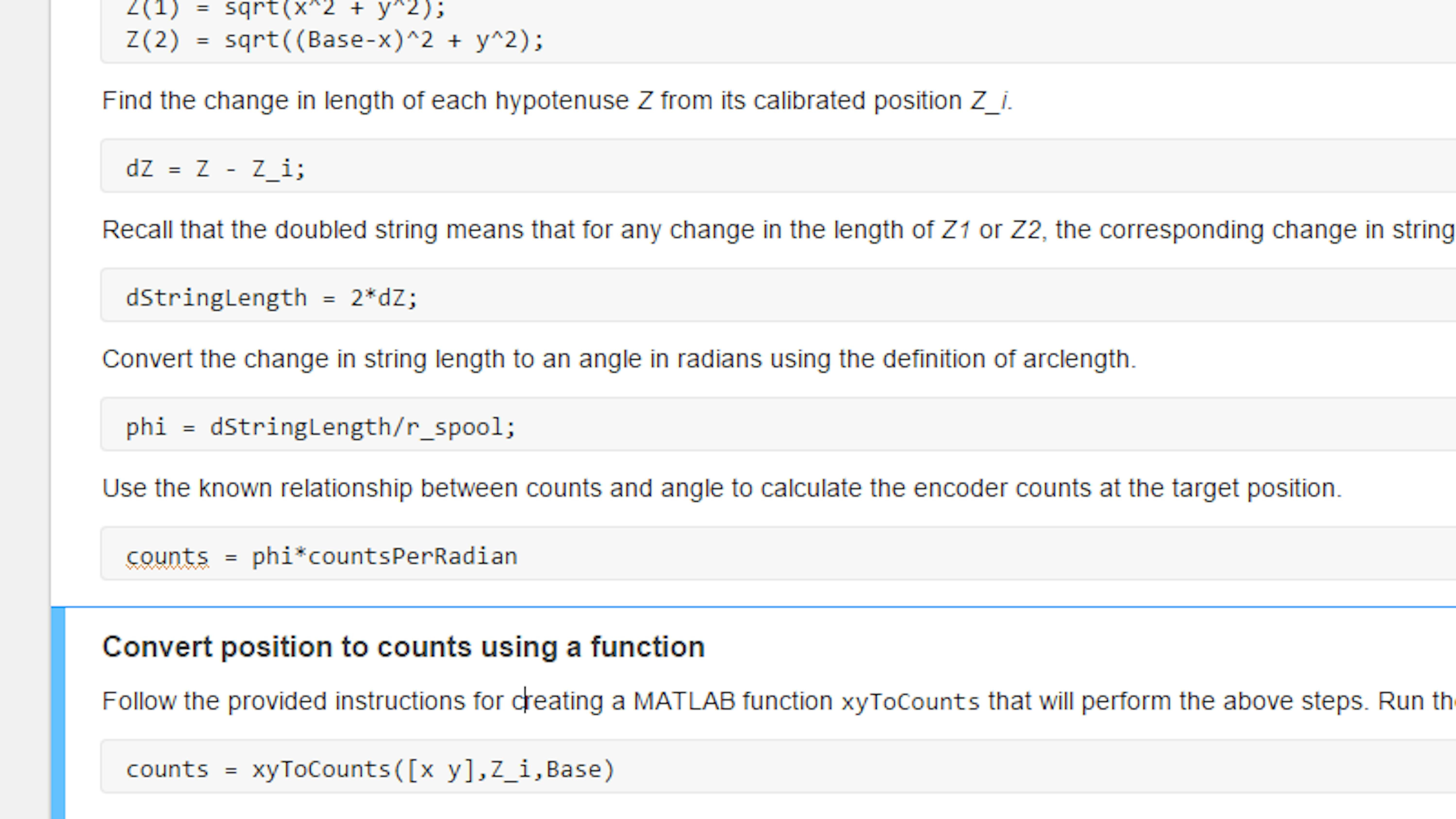
${\Delta}Z=Z-Z_i$
${\Delta}{StringLength}=2{\cdot}{\Delta}Z$
The arclength definition allows you to convert change in length to a change in angle around the motor spool.
$\theta =\frac{{\Delta}{StringLength}}{r_{{spool}}}$
Finally, use the known ratio of counts per radian to compute the desired count value for each motor.
$C=\theta {rad}{\cdot}C_{{rad}}\frac{{counts}}{{rad}}$
To perform these calculations in code, run the sections of code under the Convert target position to encoder counts heading in Task3.mlx.
WRITE A FUNCTION FOR CONVERTING POSITION TO MOTOR COUNTS
As you did in the previous exercise, you can take code you've written to solve a specific problem and encapsulate it in a function. Just as you did for converting counts to position, you can now write a function that converts position to counts. Create a new function called xyToCounts.m and include the following code.
function counts = xyToCounts(xy,Z_i,Base)
% Define constants
r_spool = 0.0045;
countsPerRevolution = 1200;
countsPerRadian = countsPerRevolution/(2*pi);

% Convert x and y to Z1 and Z2
x = xy(:,1);
y = xy(:,2);
Z(:,1) = sqrt(x.^2 + y.^2);
Z(:,2) = sqrt((Base-x).^2 + y.^2);
% Subtract initial Z to get change in Z
dZ = Z - Z_i;
% Convert change in Z to change in string length
dStringLength = 2\*dZ;
% Compute change in string length to angle
phi = dStringLength/r_spool;
% Convert angle to counts
counts = phi\*countsPerRadian;
Note that there is a slight difference between the code in this function and the code that you executed in Task3.mlx. Here, we index the xy and Z variables with subscripted indices (:,1) and (:,2) in the following lines:
x = xy(:,1);
y = xy(:,2);
Z(:,1) = hypot(x,y);
Z(:,2) = hypot(Base-x,y);
This syntax allows you to refer to all the values in the first or second column of these variables respectively, which enables you to use the xyToCounts function on not just one x-y coordinate, but on a set of x-y positions defined in an Nx2 array where the first column has all the x-positions and the second column has all the y-positions. You'll get to apply an example of this at the end of this exercise. Save the function xyToCounts.m and then test it out by running the section of Task3.mlx with the header Convert position to counts using a function . Make sure that the values for counts are the same values you obtained previously. This will prove that your function works as expected.
CONCEPT: FOR LOOPS, IF STATEMENTS, AND BREAK
There are several kinds of flow control structures that are important to understand when writing code. In this section, we'll review for loops, while loops, if statements, and the break keyword. A for loop is used when you want to run a section of your code for a predetermined number of times. If you know that you want to run a loop 5 times, you can write a for loop with a looping variable that ranges from 1 to 5. Consider the following code:
for ii = 1:5
	disp("Iteration " + ii)
end
Create a new MATLAB file, and run the above code in MATLAB. You'll see the following output.
Iteration 1
Iteration 2
Iteration 3
Iteration 4
Iteration 5
Now imagine you don't know in advance how many times you wish to repeat your code. Perhaps you want to run something until some condition is met. You can use a while loop to do this. The condition of a while loop is defined with logical expressions. Run the following code at the MATLAB Command Prompt to see how these logical expressions work.
>> x = 1
>> x > 64
>> x = 100
>> x > 64
You should see the following output.
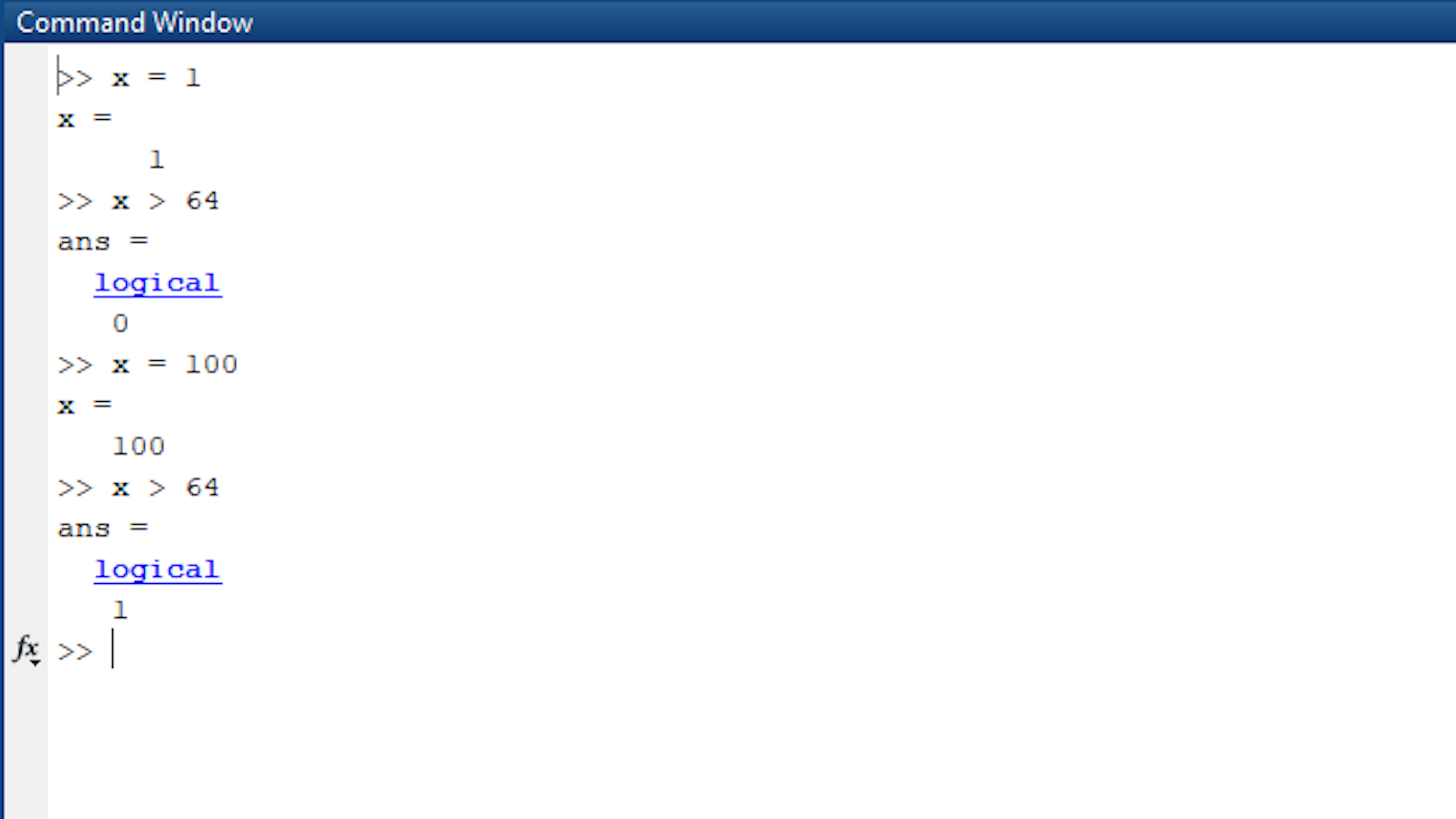
A logical expression in MATLAB is one that returns a logical value of 1 or 0 (true or false). In a while loop, the loop will continue to run as long as the condition is returning 1 (true). If the condition fails and returns 0 (false), the loop will end. In the code file where you wrote a for loop, replace the code with the following:
x = 1;
while x < 64
	x = x\*2;
	disp("Current value of x: " + x)
 end
Now, instead of running the loop a specified number of times, you're running it until the logical condition x < 64 ceases to be true. Run this code in MATLAB. You should see the following output:
Current value of x: 2
Current value of x: 4
Current value of x: 8
Current value of x: 16
Current value of x: 32
Current value of x: 64
An if statement is another flow control structure that checks a logical condition. It will execute its contents once if the condition is true and will not execute if the condition is false. Replace your while loop with the following code. Change the first line to different values and run the code to see when the display line does or does not execute.
x = 1;
if x > 5
	disp("x = " + x + " passed the test")
end
Change the value of x to 6 and run the code again. What output do you see?
A while loop will check its condition every time it reaches the end of the loop and starts over. Sometimes you might want the loop to exit somewhere in the middle as soon as a condition is met. You can do this with the break keyword. Update your code to the following:
x = 1;
while true
	x = x\* 2;
	if x >= 64
		break
	end
	disp("Current value of x: " + x)
end
The while loop's condition is set to true, so this loop would never exit if it didn't hit the break command. However, when the if statement's condition is met, the loop will break immediately without running the rest of the code. What do you think will be the last line of output displayed? Run the code to check your prediction.
In the next section, you'll see a function that uses these concepts to drive the whiteboard drawing robot through a set of points and exit the loop immediately when it's reached its target point.
UNDERSTAND MOVETOCOUNTS FUNCTION, LINE BY LINE
To move the robot through a series of specified positions defined in counts, the function moveToCountshas been provided for you. Read through the following description of its parts to see how it continuously measures the current position and updates the target speed of each motor, thereby moving the robot in the right direction. The values for the parameters wRefand hitRadius worked well with the robot well during our tests. You can edit the function and adjust these to tune the robot for your environment using these values as a starting point.
This function takes a list of encoder counts to move the robot to. It also uses the variables for existing
motor and encoder objects.


function moveToCounts(counts,m1,m2,e1,e2)
Set a target angular velocity for the motors, wRef. Set a maximum distance to the target point, hitRadius.
Start the motors.
wRef = 20; %rpm
hitRadius = 20; %counts
start(m1)
start(m2)Set up a for loop that moves through all target points. In each iteration, define the target point as countTarget.
% Loop through all points
nPoints = size(counts,1);
for ii = 1:nPoints
% Determine destination point
countTarget = counts(ii,:);Use a while loop to keep moving the robot until it's at the target point. In this loop, first measure
the current position.
% Loop until at destination
while true
% Update count measurement
countNew = [readCount(e1) readCount(e2)];Compare the current position to the target position. If the distance is less than hitRadius, break out of
the while loop immediately.
% Check distance to final position and break if close enough
countRemain = countTarget - countNew;
countNorm = sqrt(sum((countRemain).^2));
if countNorm <= hitRadius
break
endIf the robot is not yet at the target point, normalize the remaining distances and scale by the target speed.
Apply these speeds to each motor with the setSpeed method.
% Compute and set target angular speed for each motor
wSet = (countRemain/countNorm)*wRef;
stop(m1),start(m1),setSpeed(m1,round(wSet(1)));
stop(m2),start(m2),setSpeed(m2,round(wSet(2)));
endWhen all target points have been reached, end the for loop and stop the two motors.
end
stop(m1)
stop(m2)
endMOVE ROBOT TO TARGET POSITION
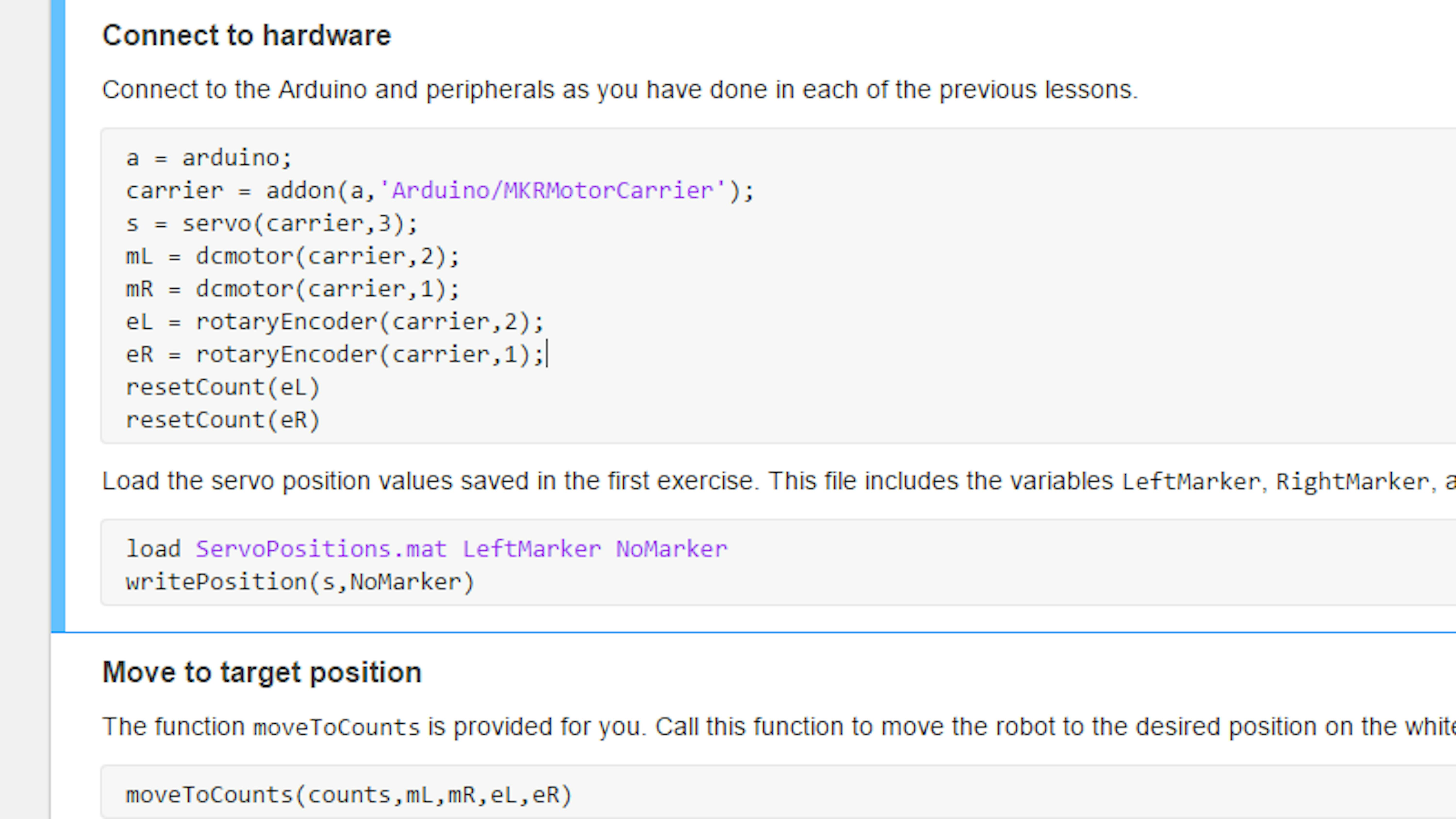
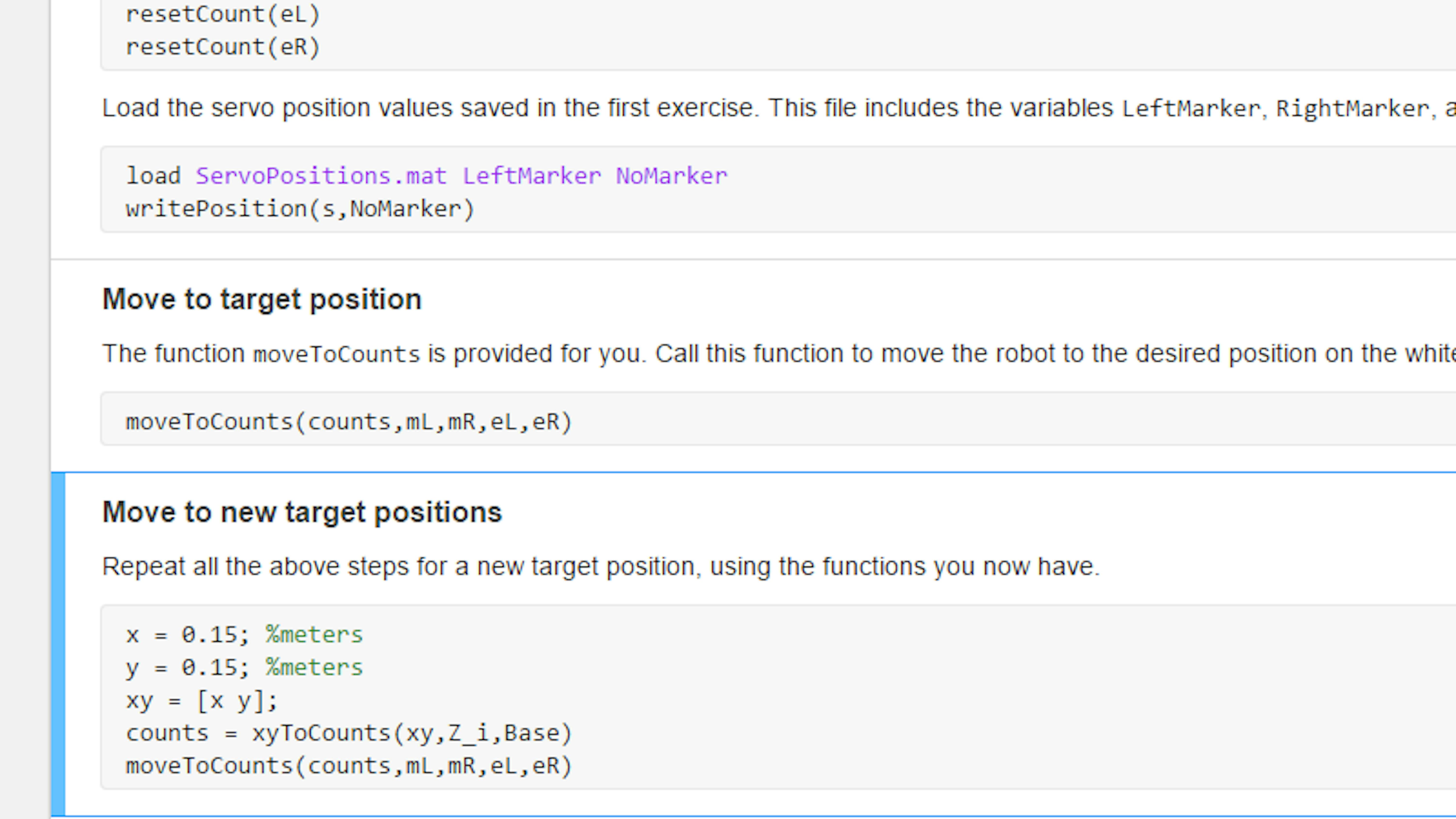
Connect to the hardware, motors, and encoders from MATLAB. Then use the moveToCounts function to move the robot to your desired x-y position. To do this, run the code in the Connect to Hardware and Move to target position sections of Task3.mlx.
MOVE TO A NEW TARGET POSITION
You can now direct the robot to move to different parts of the board. This only takes a few lines of code now that you have the xyToCounts and moveToCounts functions. In the section of code called Move to new target position , choose new values for x and y . Run this section to move the robot there. You can do this multiple times with other x and y positions.
MOVE TO A SEQUENCE OF POSITIONS
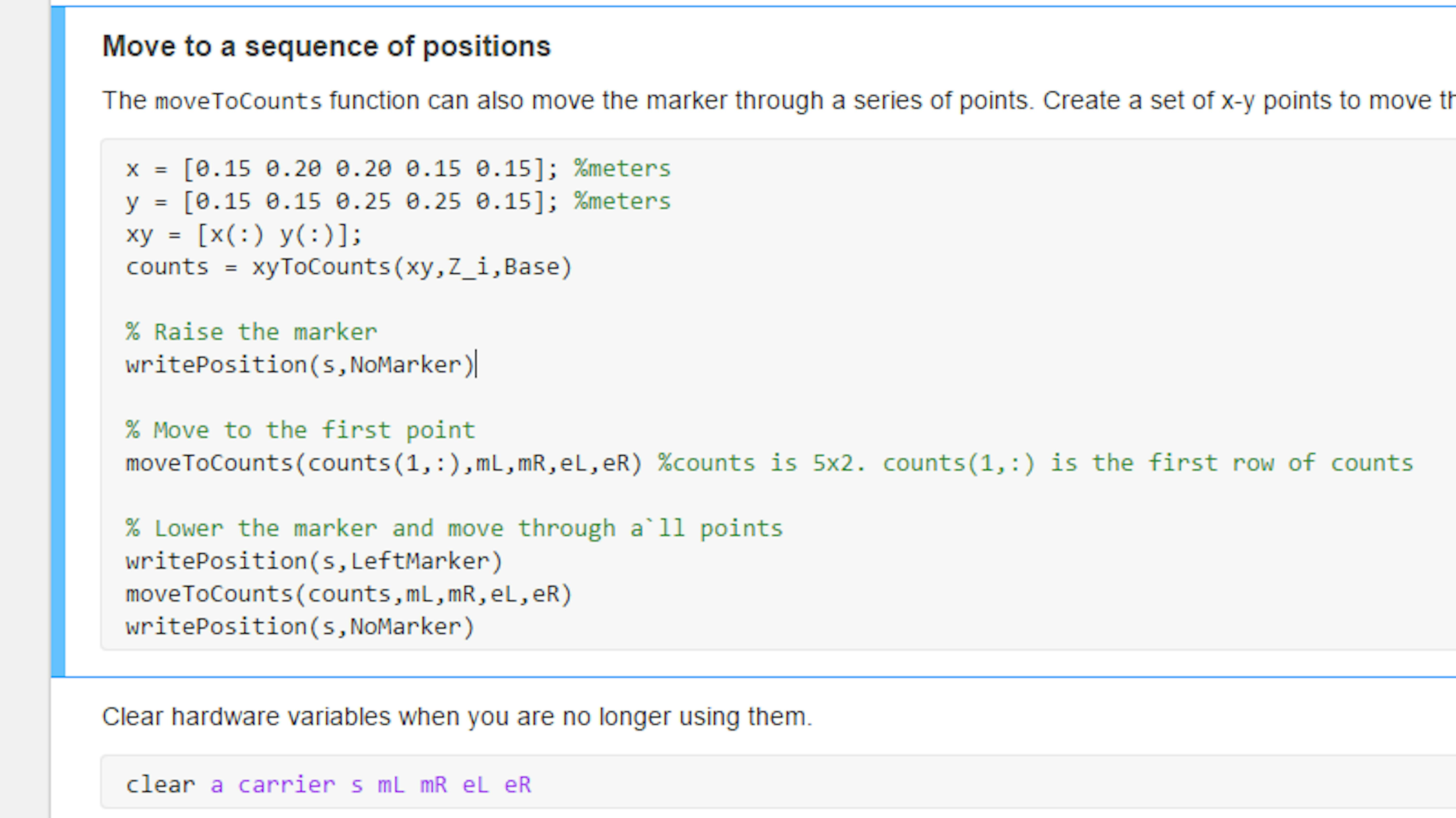
The functions xyToCounts and moveToCounts are also able to take lists of points. If you define your target x-y points as an Nx2 array where the first column is the x -coordinates and the second column holds the y -coordinates, you can direct the robot to move to a series of points. The Move to a sequence of positions section of Task3.mlx has an example of coordinates that form a rectangle. Check whether these points fall in the drawable area of your whiteboard and change them if they do not. Notice that this code also includes a sequence of actions required for drawing shapes. It raises the marker, moves to the first point, lowers the marker, moves through all the points, and raises the marker again.
Run this section of code.
FILES
- Task3.mlx
- xyToCounts.m
- moveToCounts.m
LEARN BY DOING
In the last section of this exercise, you saw how you could raise and lower the marker between moving to positions. Try to draw a multi-line segment with this approach, raising the marker between lines. Draw a capital letter E. Define the coordinates of all the six segment endpoints. You can draw the three outer segments together, then raise the marker and draw the middle line.
In MATLAB, use the equation of a circle to define x-y positions for eight points on a circle. (This will form an octagon.) Draw this shape on the whiteboard.
EXERCISE 4:
4.4 Identify position limits
If you try to move the robot to the top of the whiteboard, it won't have enough power to move above a certain point. If you try to move it too close to the pulleys, it will collide with them and get stuck. At the bottom of your whiteboard, there may be a marker tray you don't want the robot to run into. In this exercise, you determine what parts of the whiteboard the robot can reach and what parts you shouldn't try to move the robot to.
You'll learn about important concepts in physics that will help you determine how much load the motors are under at any point on the whiteboard. Then you'll do the computations yourself and create visualizations to see how much load there is at every position and where the load is greatest.
In this exercise, you will learn to:
- Apply motor stall equations
- Use symbolic math API to convert units
- Create free-body diagrams
- Compute forces on static body
- Apply a function at every point on a grid
- Plot surfaces and images in MATLAB
UNDERSTAND MOTOR EQUATIONS AND STALL CONDITIONS
For a DC motor, a mathematical equation can be used to describe the relationship between motor load (torque), supply voltage, and rotational speed. This is sometimes referred to as the DC motor torque equation:
$\tau =\frac{V-{\omega \cdot k}} R{\cdot}k$
In this equation, $\tau$ is the motor torque or motor load, V is the supply voltage, and $\omega$ is the angular speed. (Note that in some versions of this equation, the variable T is used for torque. For our project, we'll reserve T to use for tension.) R is the resistance in the motor windings, and k is the motor constant. Both R and k are constant for a given motor. There are two special cases we can consider for this equation. One is the case where there is no load on the motor. In this case, $\tau$ = 0, and the equation simplifies to the following:
$V=\omega _{{free}}\cdot k$
The second special case is when the motor reaches stall conditions. This is when the load is so high that the motor cannot spin. In this case, $\omega$ = 0, and the equation simplifies to the following:
$\tau _{{stall}}=\frac{{Vk}} R$
CALCULATE MAXIMUM ALLOWABLE LOAD
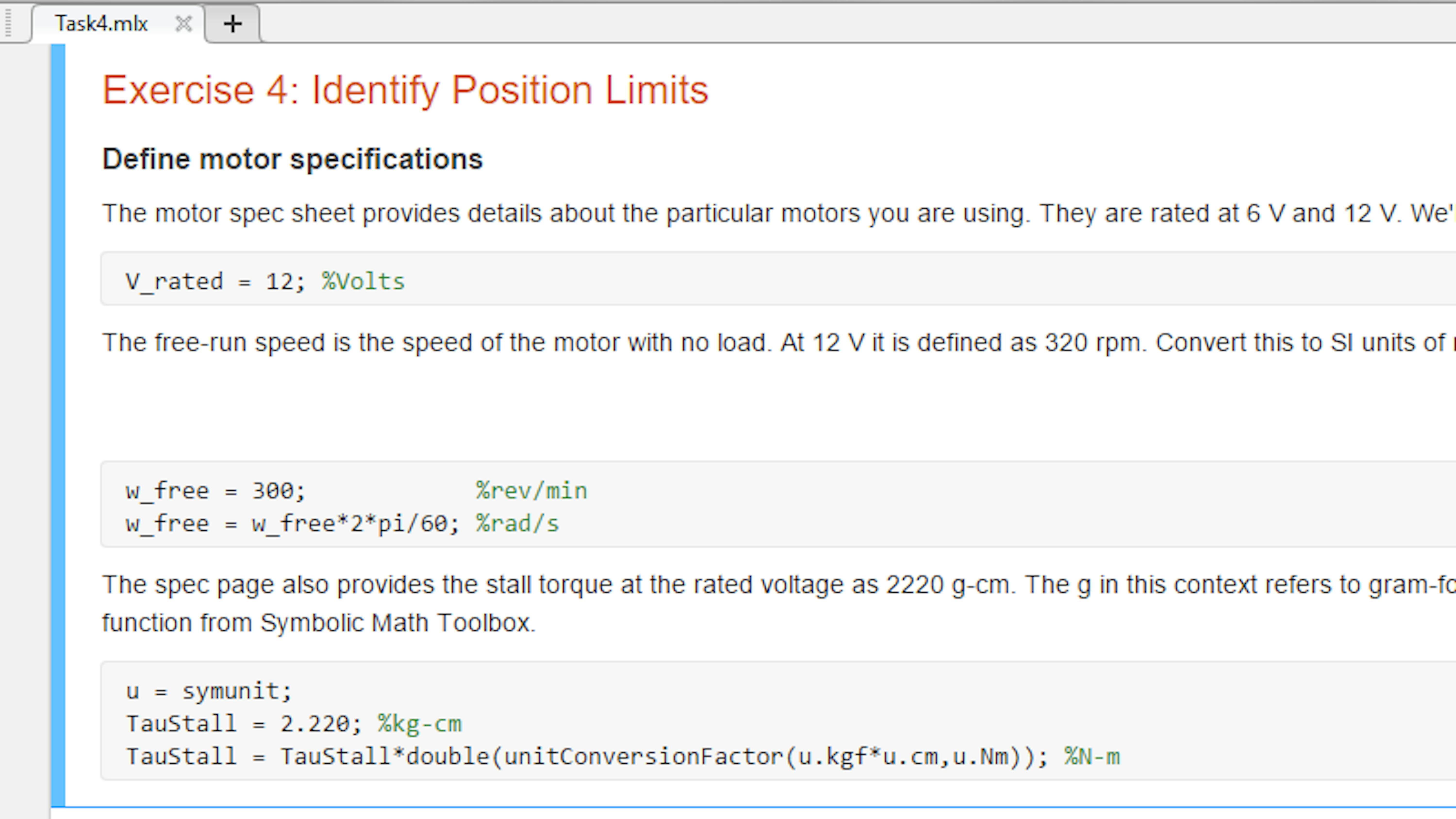
First, check out the specifications provided for the motor. They are available here or here. The motor is rated at 12 V. Record the specified voltage, free-run speed, and stall torque in code. Convert them to SI units. Symbolic Math Toolbox provides a useful function called unitConversionFactor that can give you the conversion factor to convert kg-cm to N-m. The code for these steps is contained in the live script Task4.mlx. Open this file. Then run the section of code under the heading Define motor specifications.
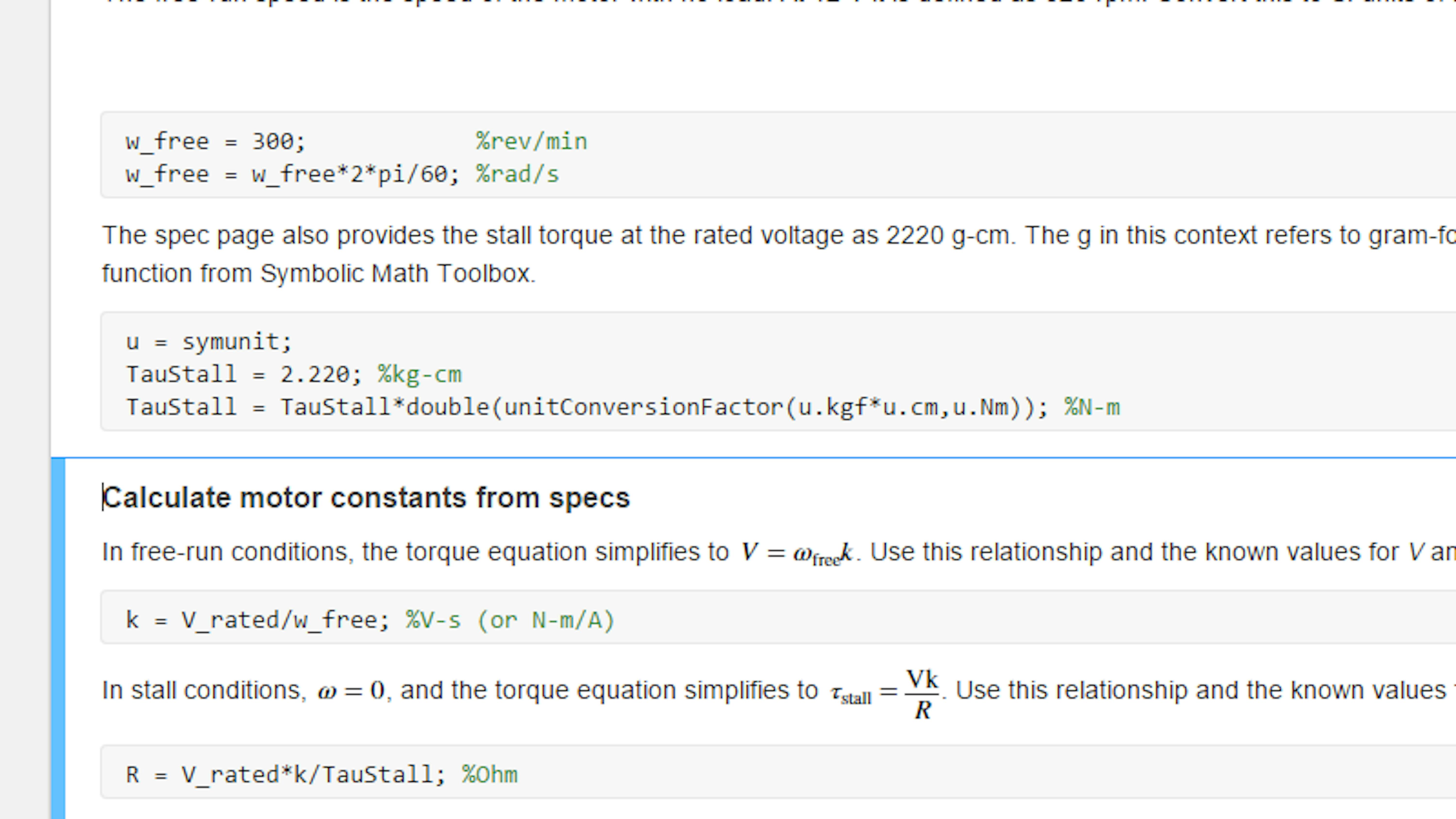
You can use the motor's voltage-speed-torque relationship to determine the constants $k$ and $R$ for the motor. First use the motor equation in free-run conditions where $\tau$ is 0 to calculate $k$ . Then use the motor equation in stall conditions where $\omega$ is 0 to calculate $R$. Run the section of code under the heading Calculate motor constants from specs in Task4.mlx.
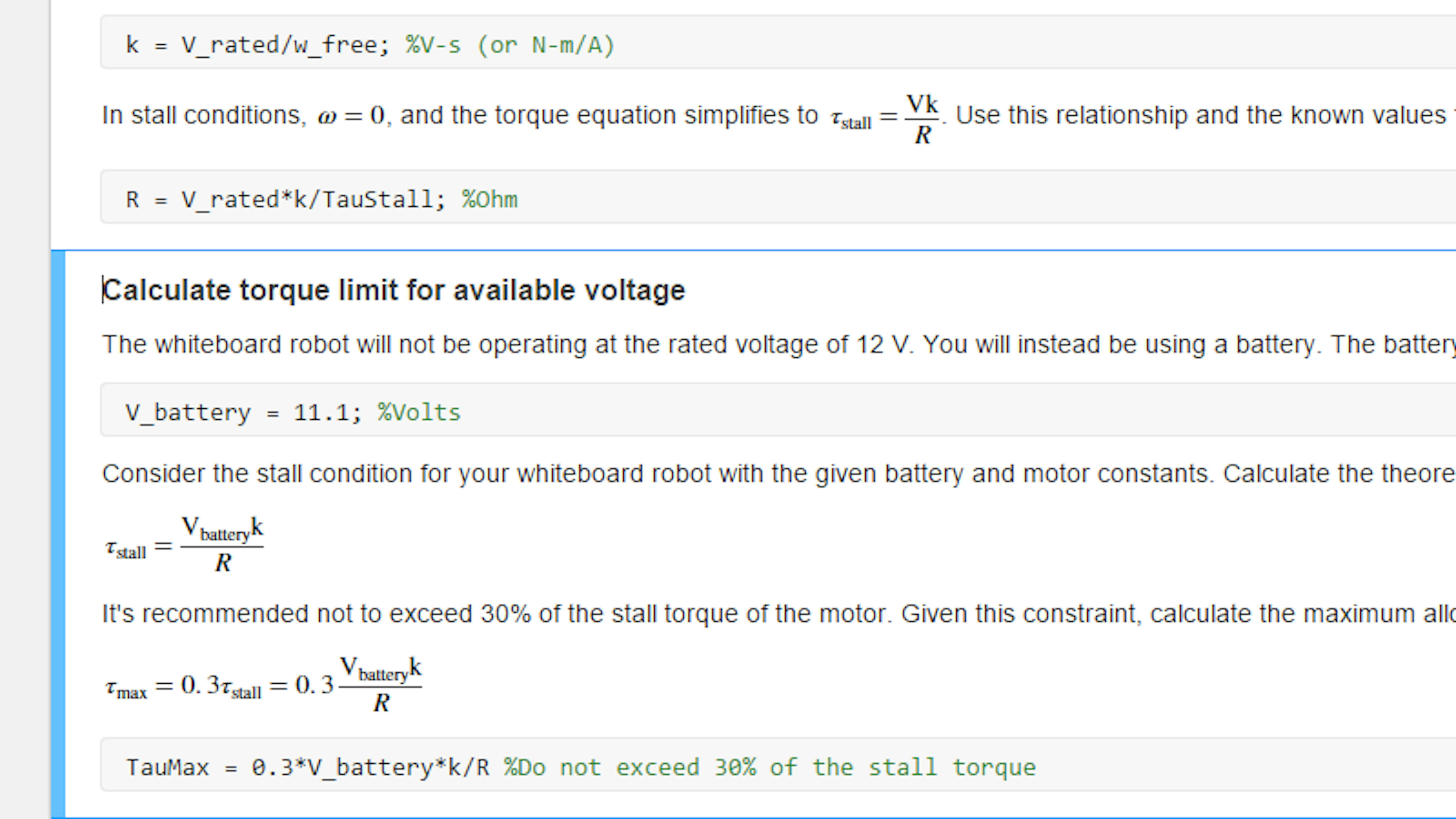
Your robot will not be running the motors at the rated voltage. Instead, in the kit, you have a battery with a rating of 11.1 V. This will put a restriction on the stall toque for your operating conditions. Also, it's good practice not to run the motor at more than 30% of the stall torque , more information here or here . Use the motor equation under stall conditions to calculate the stall torque given your battery, then choose 30% of this value as the maximum allowed torque on your robot's motors. We will call this variable TauMax . To compute this value, run the section of code in Task4.mlx under the heading Calculate torque limit for available voltage.
UNDERSTAND THE FREE-BODY DIAGRAM
Think about hanging the robot at various parts of the whiteboard. Do you think the motors will have a harder time turning if they are at the top or at the bottom? Is it easier to move up or down the whiteboard? Which motor will have the greater load when the robot is all the way at the left edge of the whiteboard?
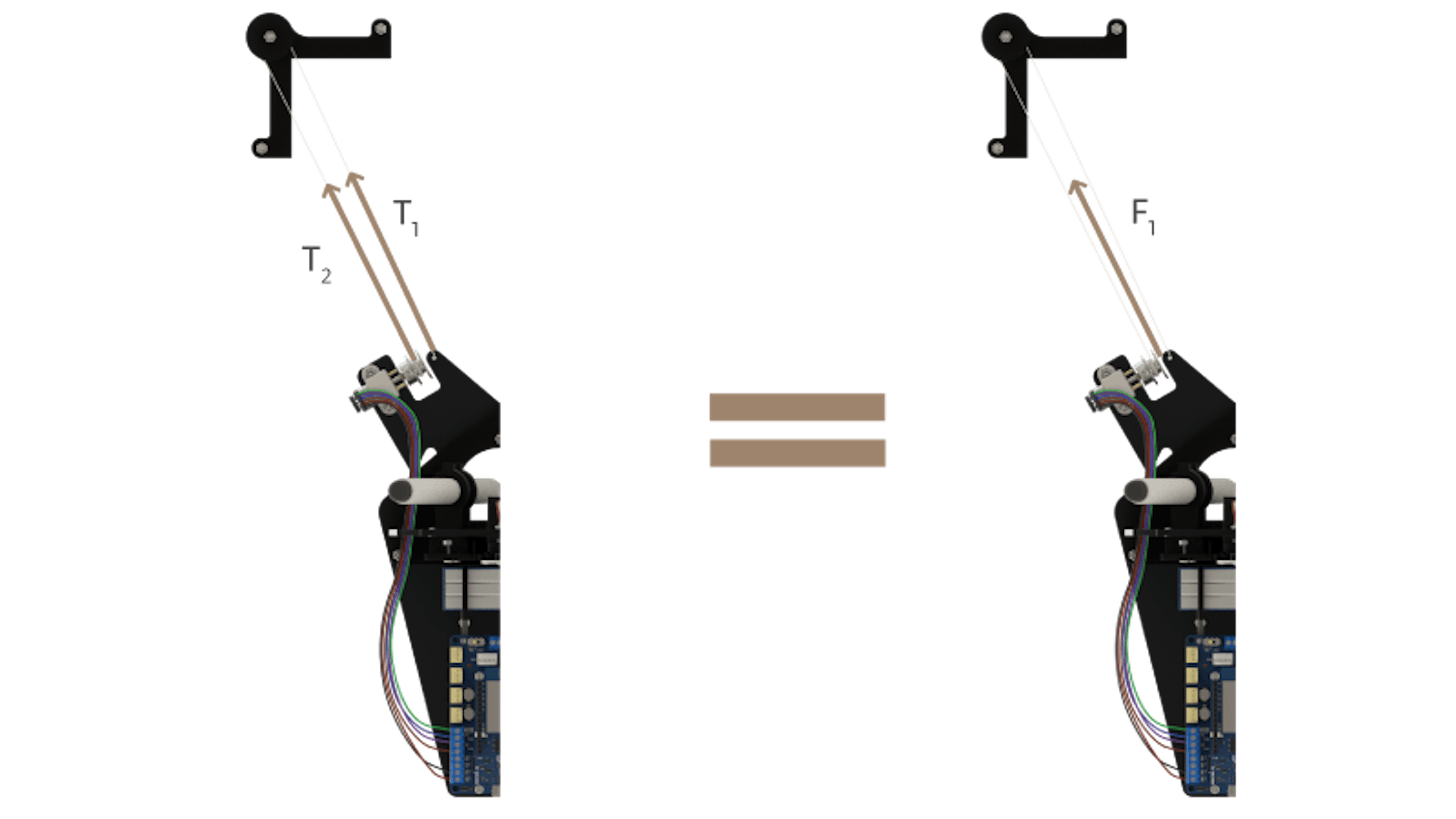
In physics and engineering it's often useful to be able to calculate the forces on an object. For the whiteboard robot, these forces can tell us how much load is on each of the motors. This is done by creating what is known as a free-body diagram , which is a diagram showing a body with forces acting on it in different directions. On the robot, there are two strings pulling toward the left pulley. These should each be pulling with the same tension $T_1$, so we can treat them as a single force $F_1$ whose value is twice $T_1$. Similarly, the two strings pulling toward the right pulley $T_2$ can be treated as a single force $F_2$, where $F_2 = 2 \cdot T_2$. Finally, there is a weight pulling downward.
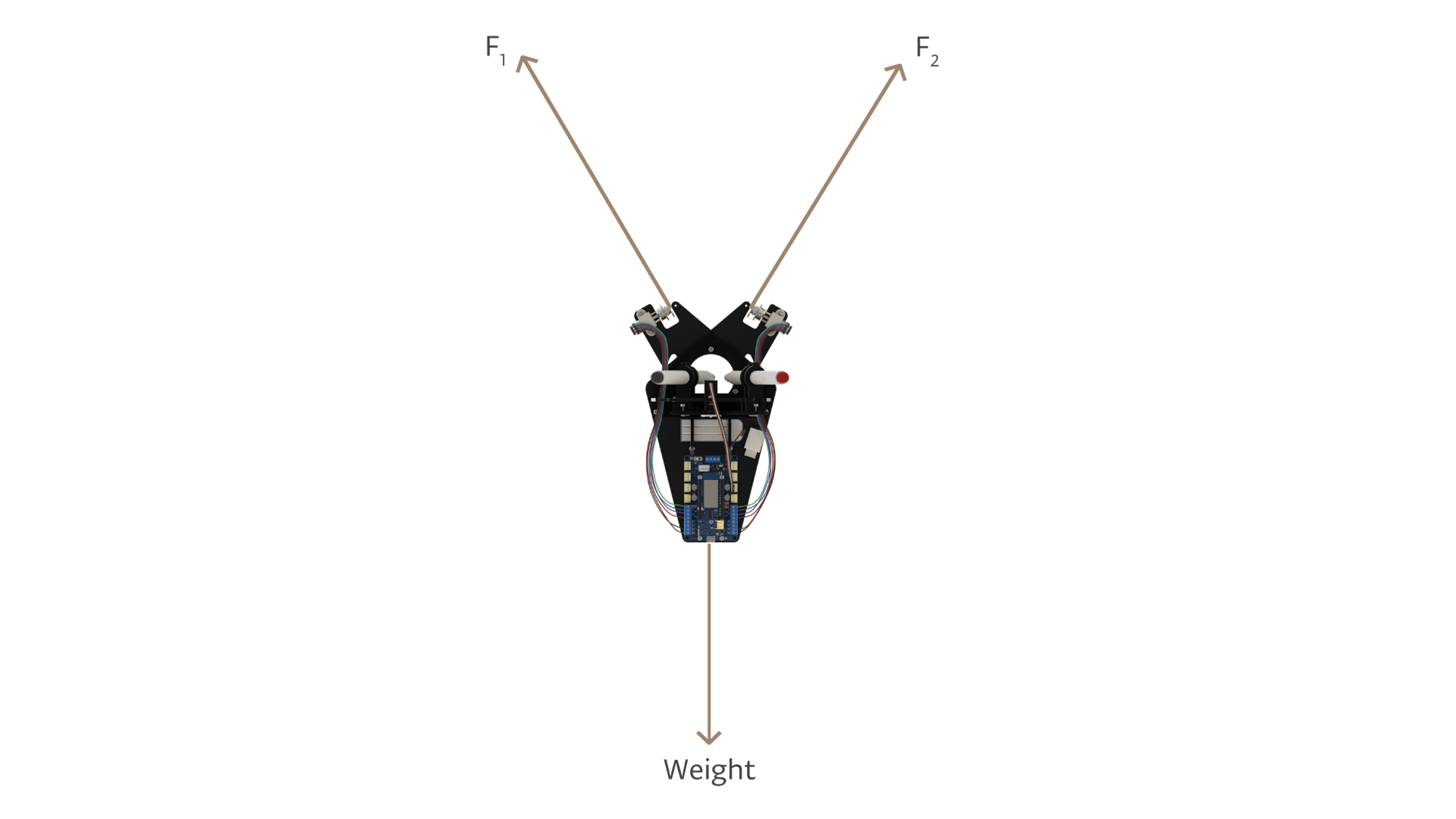
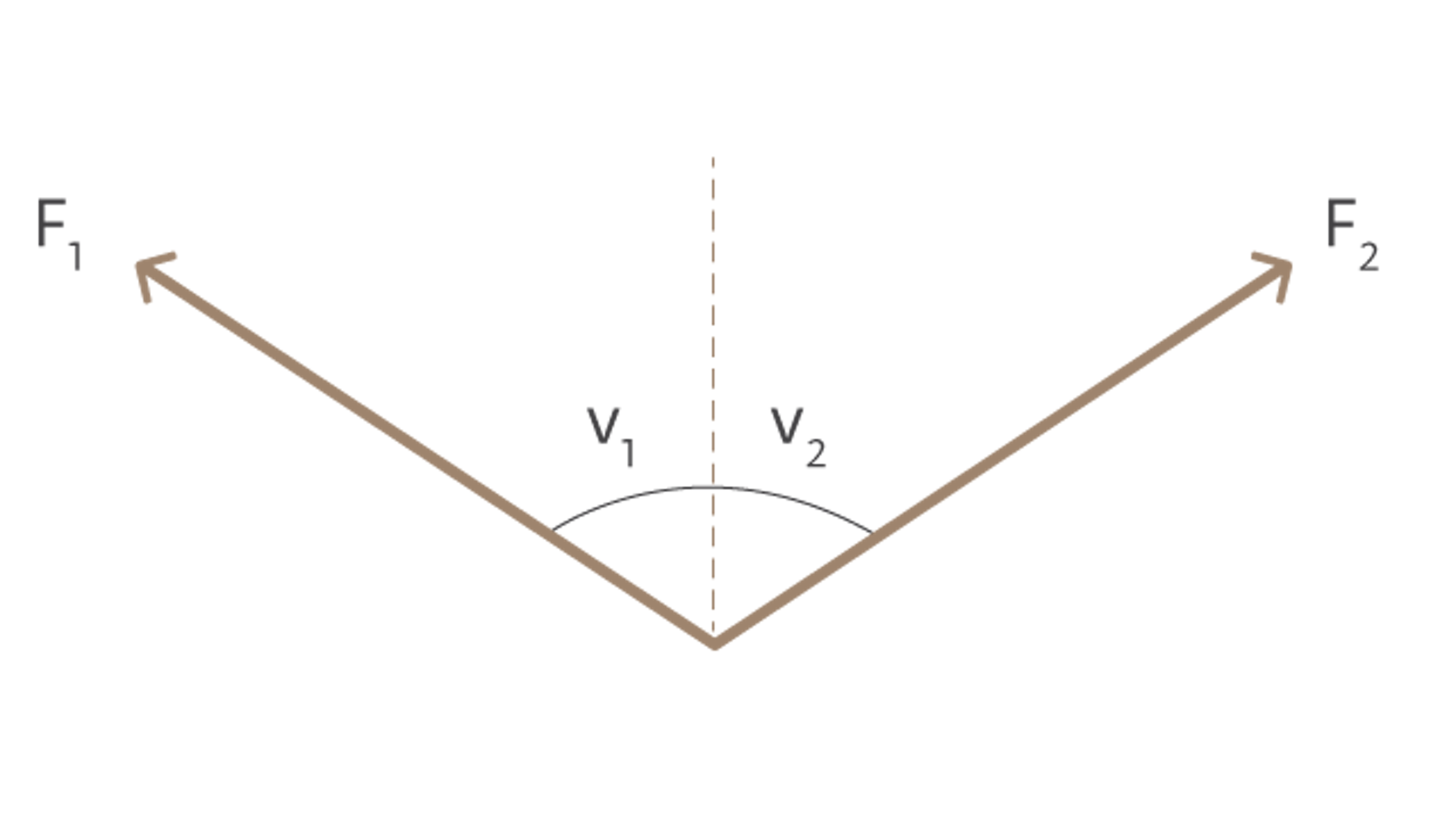
On a free-body diagram, it is also useful to break the forces down into their x and y components. First, define $\theta_1$ as the angle of $F_1$ from vertical and $\theta_2$ as the angle of $F_2$ from vertical, as shown in the following diagram. The relationship between $F_1$,$F_2$, and Weight will be explained in the subsequent sections; for now, let's focus on how to express the values of those forces in terms of the angles of the strings, which depend on the robot's location on the whiteboard.
Then use trigonometry to break each force $F_1$ and $F_2$ down into its x-component and y-component, as shown.
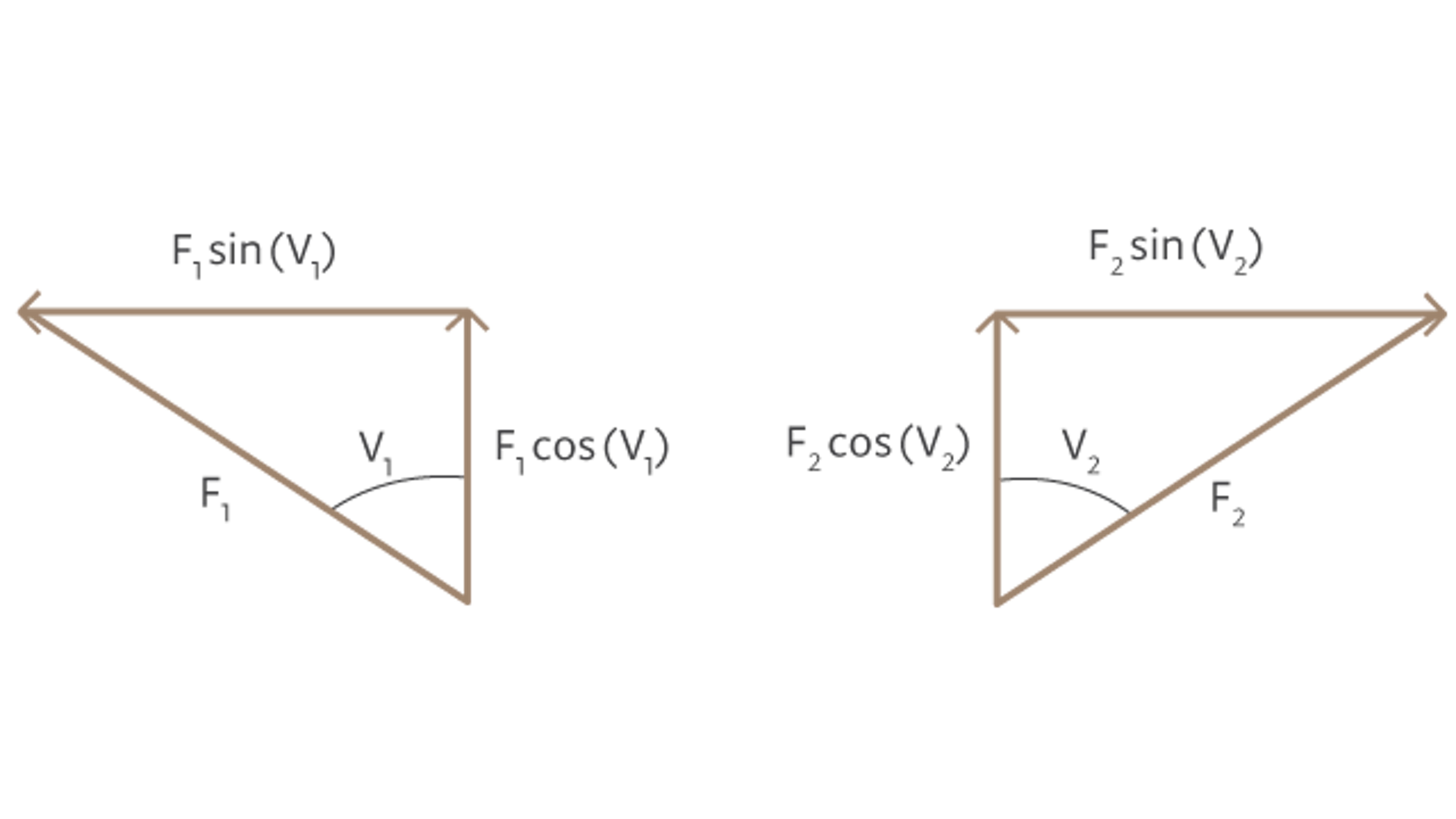
$F_{1,x}=-F_1\sin \theta _1$
$F_{1,y}=F_1\cos \theta _1$
$F_{2,x}=F_2\sin \theta _2$
$F_{2,y}=F_2\cos \theta _2$
Once you have these equations, it is fairly easy to answer the question of whether the motors will suffer the same forces at different parts of the whiteboard, at least under steady-state. The next section will cover this case.
UNDERSTAND FORCE BALANCE ON A STATIC BODY
Newton's third law of motion tells us how an object behaves with forces acting on it. The sum of the forces acting on the object is equal to the mass of the object times the acceleration of the object.
$\Sigma \overrightarrow F=m\overrightarrow a$
This equation can be broken into its component dimensions, in this case x and y.
$\Sigma F_x=ma_x$
$\Sigma F_y=ma_y$
When the robot is not moving, the acceleration in every direction is zero. This means the left side of each equation is the sum of the forces in that direction and the right side of the equation is 0. For the whiteboard robot, this gives the following two equations.
$-F_1\sin \theta _1+F_2\sin \theta _2=0$
$F_1\cos \theta _1+F_2\cos \theta _2-{Weight}=0$
Solving this system of equations algebraically for the unknown forces $F_1$ and $F_2$ gives the following:
$F_1={Weight}{\cdot}\frac{\sin \theta _2}{\sin \theta _1\cos \theta _2+\sin \theta _2\cos \theta _1}$
$F_2={Weight}{\cdot}\frac{\sin \theta _1}{\sin \theta _1\cos \theta _2+\sin \theta _2\cos \theta _1}$
Up to now, we've explored the relationships between the geometry of the robot and the various forces on the robot. However, the motor's equations are expressed in terms of torque, not force. In the next section, we'll bring together all the equations we have so far and introduce a relationship between torque and force that will tie everything together. This will allow you to determine how much load the motors are under at every point on the whiteboard.
DERIVE EQUATIONS TO COMPUTE TORQUE FROM X-Y POSITION
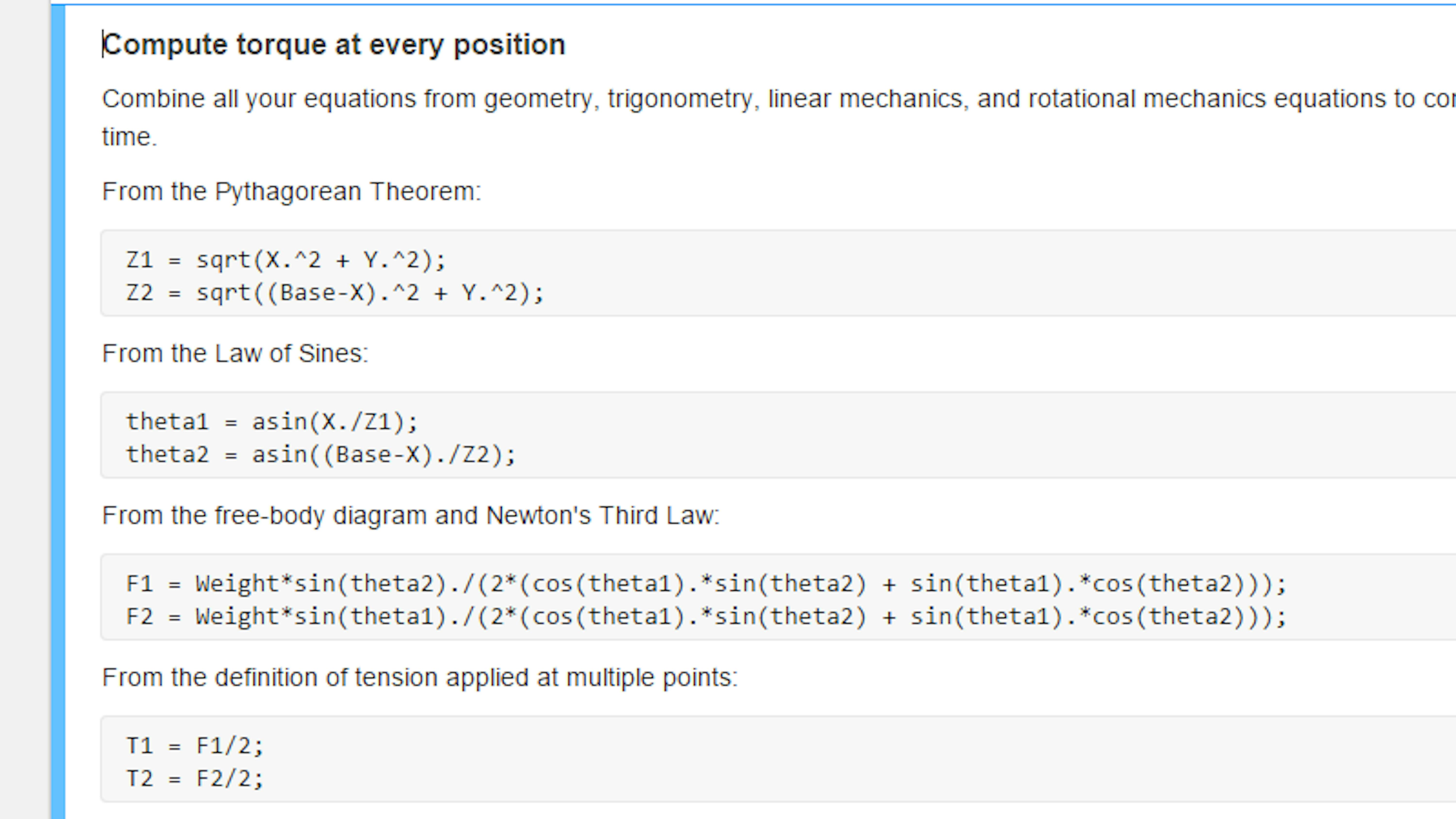
For any x, y position on the whiteboard, it is possible to compute the torque on the motor. First, use the x, y position to compute the hypotenuses of the triangles formed by the robot's hanging position, $Z_1$, $Z_2$. Use these values to compute the angles of the strings, $\theta_1$,$\theta_2$ . Then compute $F_1$, $F_2$ and $T_1$,$T_2$. Finally use $T_1$,$T_2$ to compute $\tau_1$, $\tau_2$. Here is the set of equations to use. To compute $Z_1$, $Z_2$ from x-y , simply use the Pythagorean Theorem as you have done previously.
$Z_1=\sqrt{x^2+y^2}$
$Z_2=\sqrt{\left({Base}-x\right)^2+y^2}$
To compute $\theta_1$,$\theta_2$ from x , y , $Z_1$, and $Z_2$, use the law of sines. This law states the following for any triangle:
$\frac a{{sinA}}=\frac b{{sinB}}=\frac c{{sinC}}$
In this case, we can use the relationship between the right angle of each triangle and the unknown angle $\theta$ of each triangle. This gives us the following equations:
$\frac x{\sin \theta _1}=\frac{Z_1}{\sin \pi /2}$
$\frac{{Base}-x}{\sin \theta _2}=\frac{Z_2}{\sin \pi /2}$
Since $\sin \frac \pi 2$ is equal to 1, these equations simplify to:
$\theta _1=\sin ^{-1}\frac x{Z_1}$
$\theta _2=\sin ^{-1}\frac{{Base}-x}{Z_2}$
To compute $F_1$ , $F_2$ from $\theta_1$,$\theta_2$, use the equations derived in the previous section:
$F_1={Weight}{\cdot}\frac{\sin \theta _2}{\sin \theta _1\cos \theta _2+\sin \theta _2\cos \theta _1}$
$F_2={Weight}{\cdot}\frac{\sin \theta _1}{\sin \theta _1\cos \theta _2+\sin \theta _2\cos \theta _1}$
To compute $T_1$ , $T_2$ from $F_1$ , $F_2$ , recall that the total force pulling the robot in the direction of a pulley is equal to twice the tension on the string over that pulley, because there are two points where the string pulls on the robot.
$T_1=F_1/2$
$T_2=F_2/2$
Finally, compute torque from the tension on the string. The string pulls the motor in a direction perpendicular to the line from the center of the spool to the point where the string touches the motor, as shown in the following diagram.
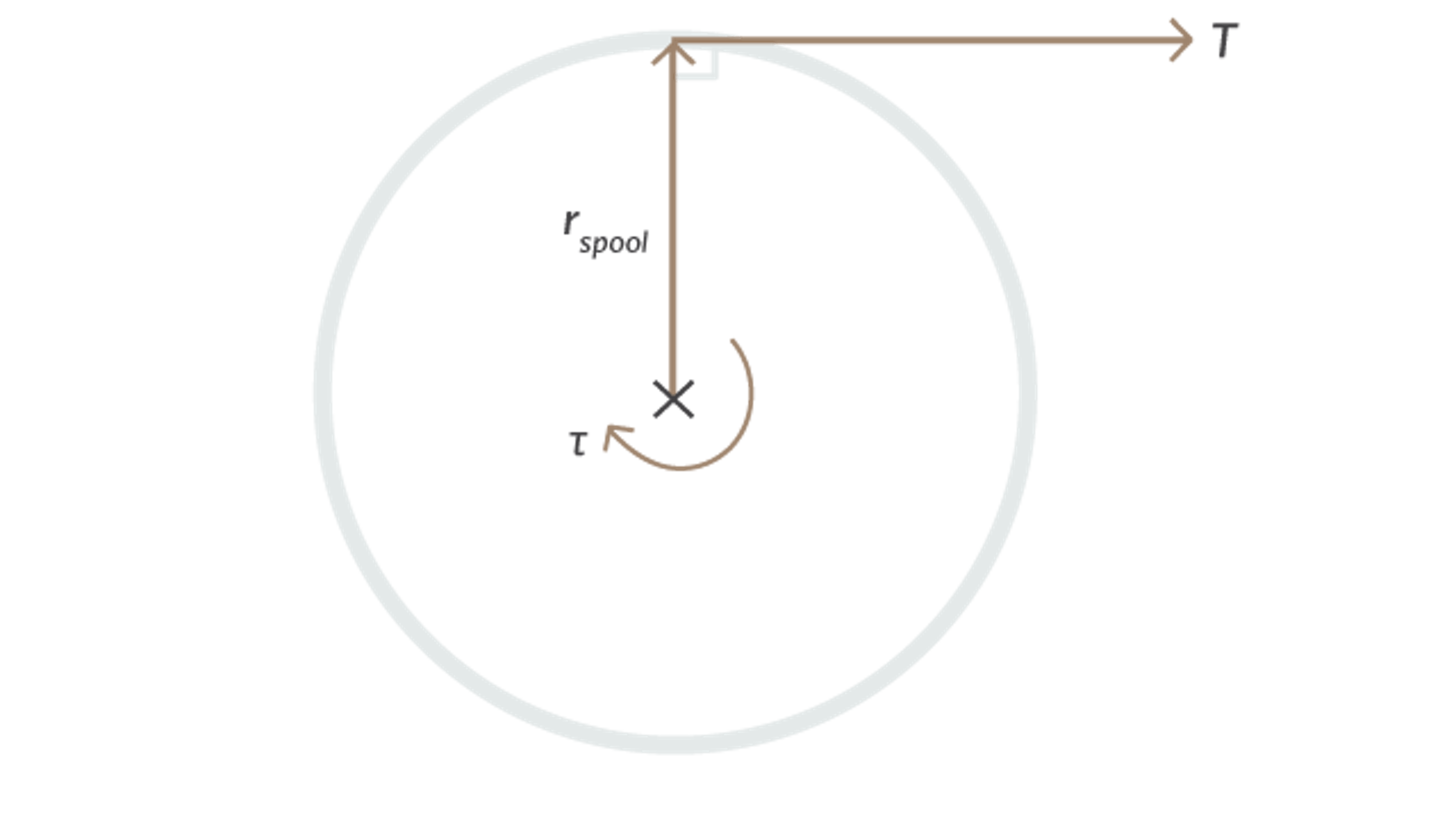
In this situation, the magnitude of the torque is given as the product of the force and the distance between the axis of rotation and the point where the force is applied. In this case, that distance is the radius of the spool, so we get the following equations:
$\tau _1=T_1r_{{spool}}$
$\tau _2=T_2r_{{spool}}$
Given all the equations introduced in this section, it is possible to compute angles in terms of location, forces in terms of angles, tension in terms of forces, and torque in terms of tension, which means there is a way to relate torque to location on the whiteboard. As you can imagine, making a map of the torques on the robot for the whole whiteboard is a long process, but having the equations and using MATLAB, these operations could be automated as shown in the following sections.
CREATE A GRID OF ALL POSSIBLE BOARD POSITIONS
To see which parts of the whiteboard the robot will be allowed to move to, you'll define a grid that covers the entire board and calculate the torque everywhere on that grid. The first step in creating this grid is to define the dimensions of the whiteboard.
Using a meterstick or tape measure, measure the height of the whiteboard, from the pulleys down to the bottom of the board. Find the section of code in Task4.mlx under the heading Define whiteboard dimensions. On the first line of code, change the value of H_board so that it is equal to your measured height, defined in meters.
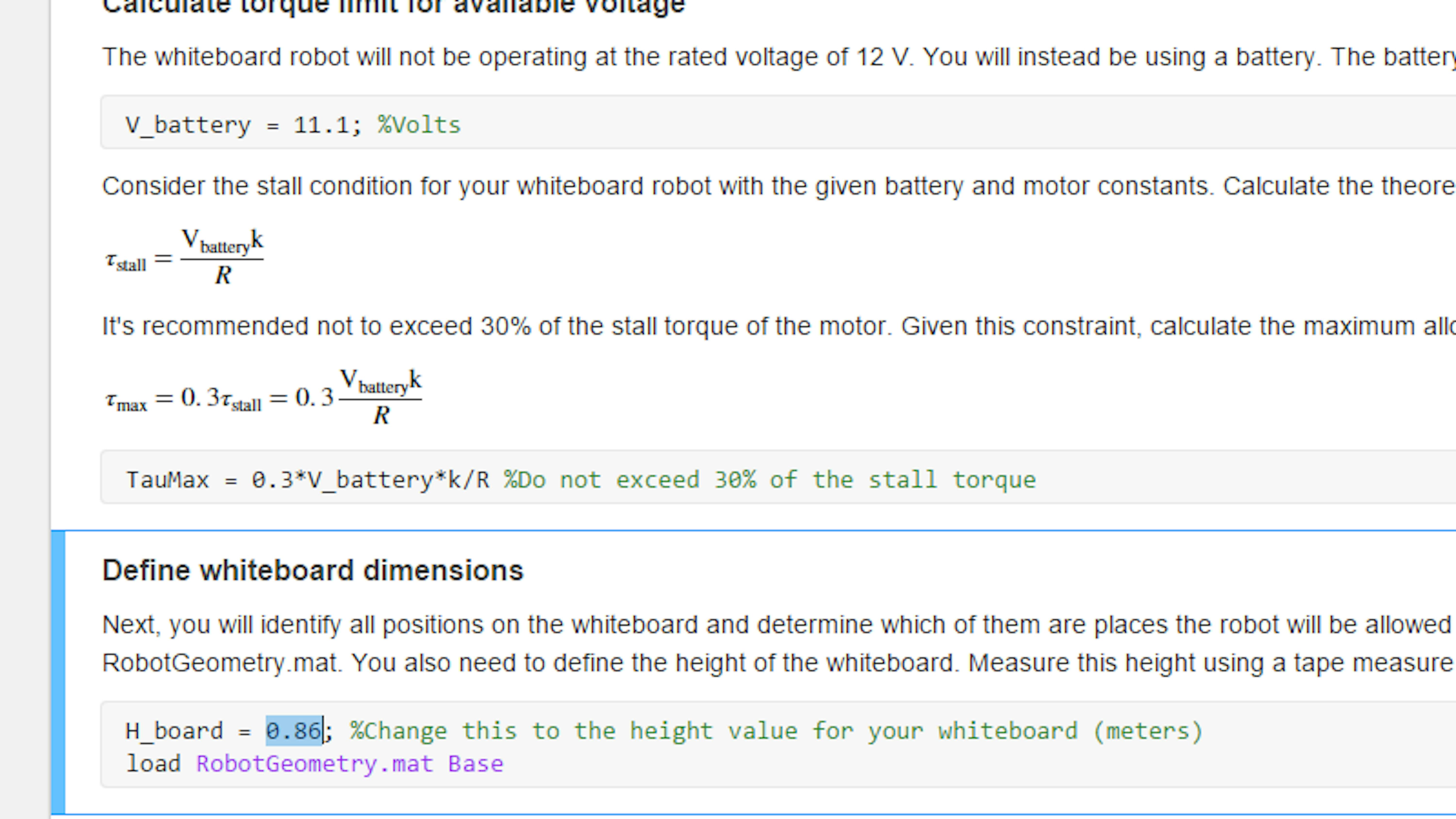
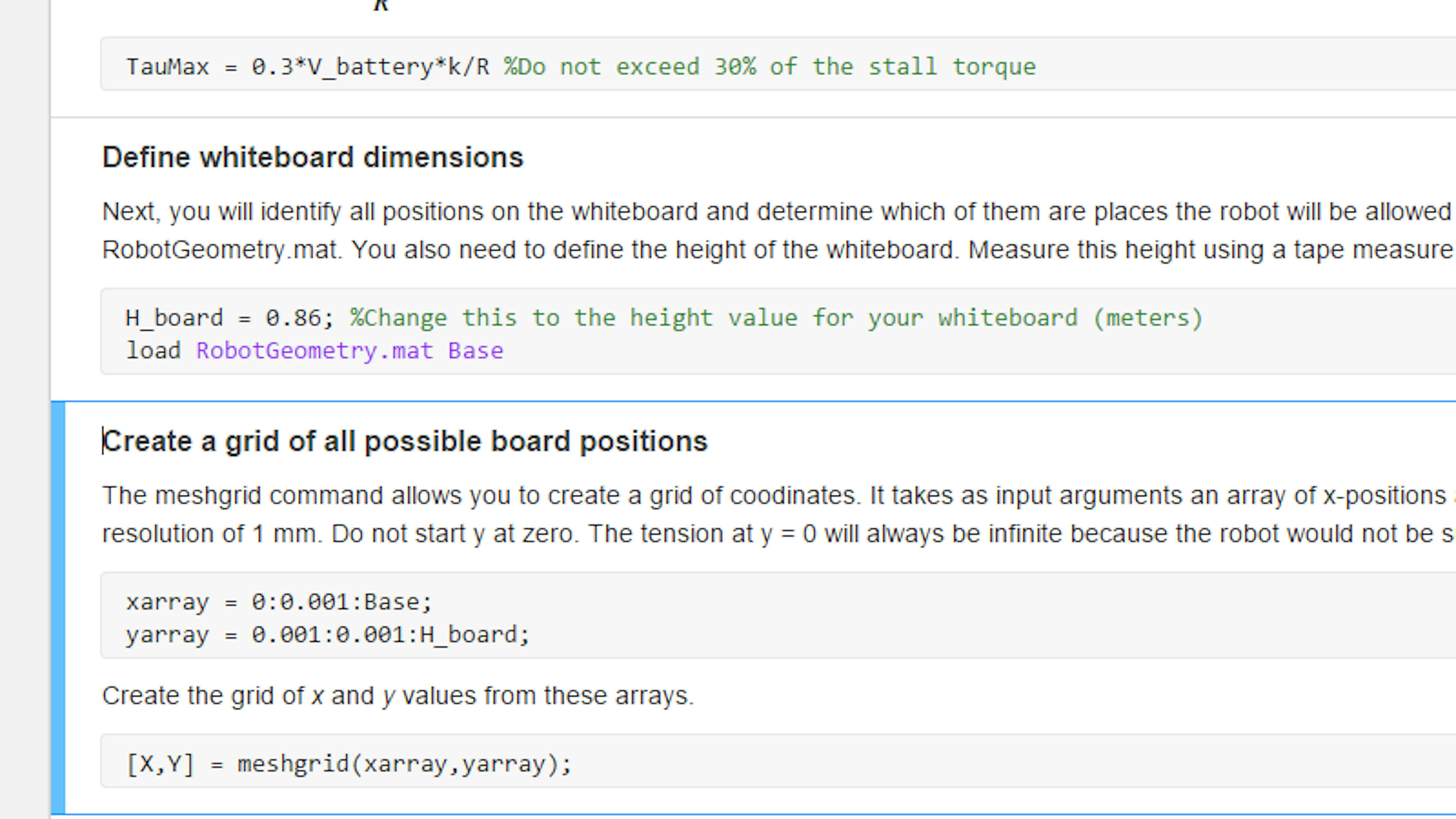
You previously measured the distance between the two pulleys. This is defined in the Base variable which you should have saved in a MAT-file. Run the Define whiteboard dimensions section of code to define the whiteboard height (H_board) and load the measured base ( Base ). A data grid of coordinate positions can be created in MATLAB using the meshgrid function. An easy way to call this function is by defining arrays of the x -values and y -values to be contained in the grid. The next section of code defines these arrays over the whole range of x and y values at an interval of 1 mm. Run the section of code under the heading Create a grid of all possible board positions in Task4.mlx.
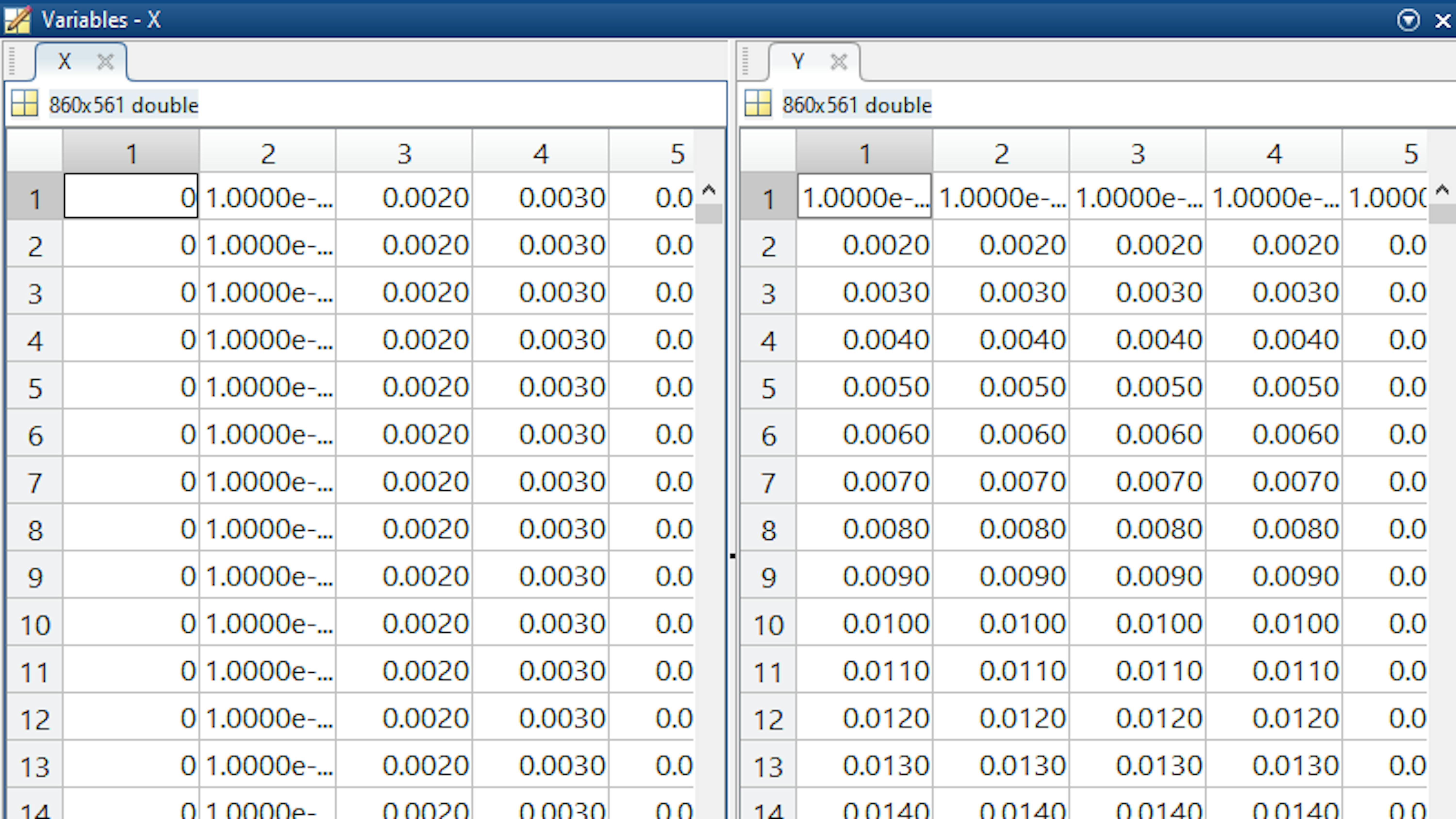
Open the variables Xand Y in the Variable Editor by double-clicking them in the Workspace. Note that they are the same size, the columns of X are all the same, and the columns of Y are all the same. Therefore, each pair of positions X(i,j) , Y(i,j) defines a unique location on the whiteboard.
We can now use these coordinate grids to evaluate the series of equations obtained earlier and visualize the results on a plot.
COMPUTE TORQUE AT EVERY POSITION AND PLOT SURFACE
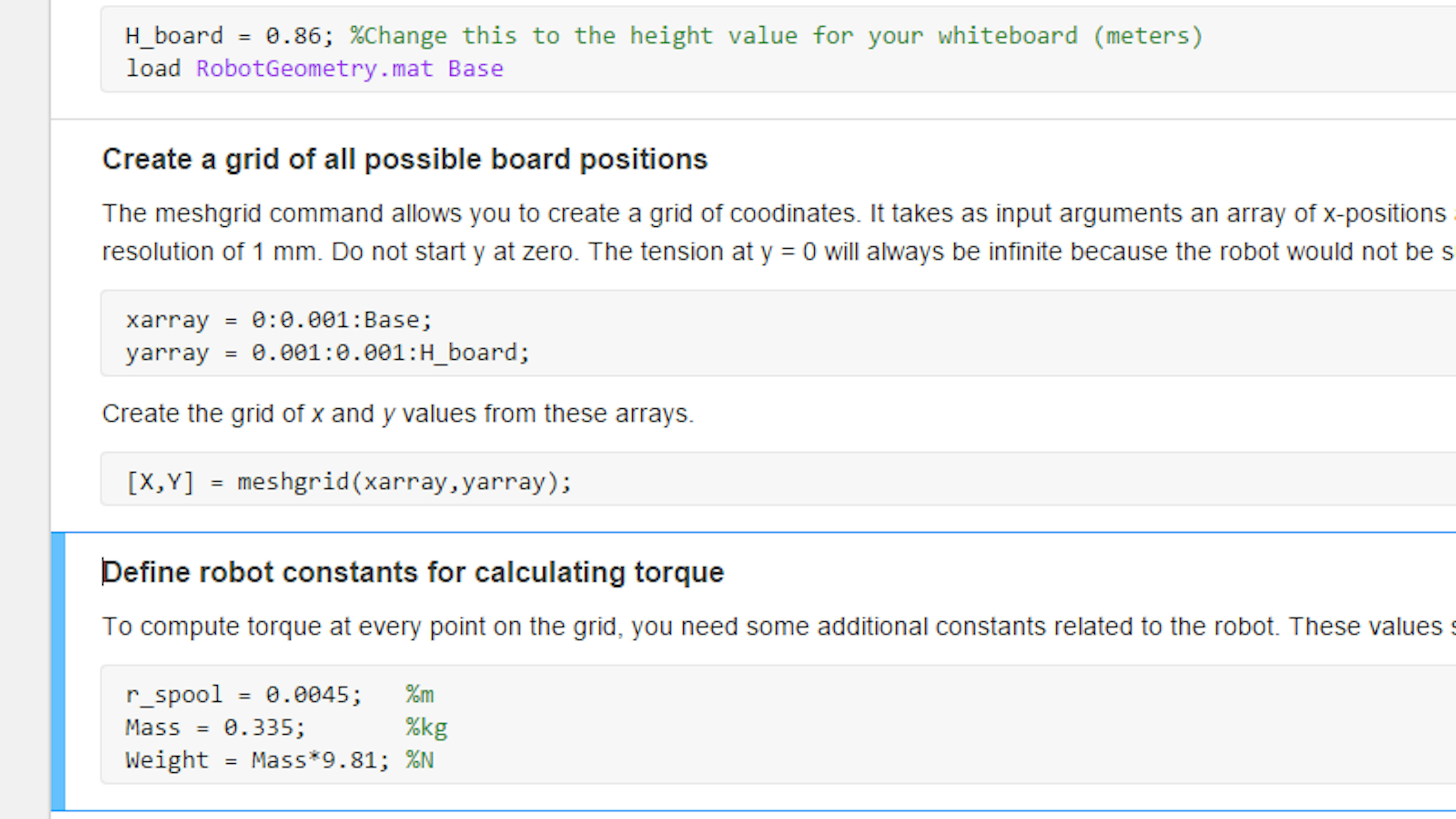
In addition to the variables currently defined, we also need to know a few additional values before we can compute the motor torques at every point on the board. To calculate the tension on each string, we need to know the robot's weight. To convert the tension to torque, we need to know the radius of the spool. These are both defined for the given robot kit. To define these in the MATLAB code, run the section of code under the heading Define robot constants for calculating torque.
Next, use MATLAB to apply the derived equations for converting x-y position to torque. First, compute $Z_1$ and $Z_2$ for every position on the whiteboard. Then apply the trigonometric equations to calculate the angles $\theta_1$ and $\theta_2$ based on the formed triangles. Use the force-balance equations to calculate the force in each direction and the tension on each string. Then compute the torque load on each motor at every position. Finally, define a single variable Tau that contains the larger of the two torque values at every position. You must never move the robot to a location where this value is greater than TauMax. Run the section of code under the heading Compute torque at every position in Task4.mlx.
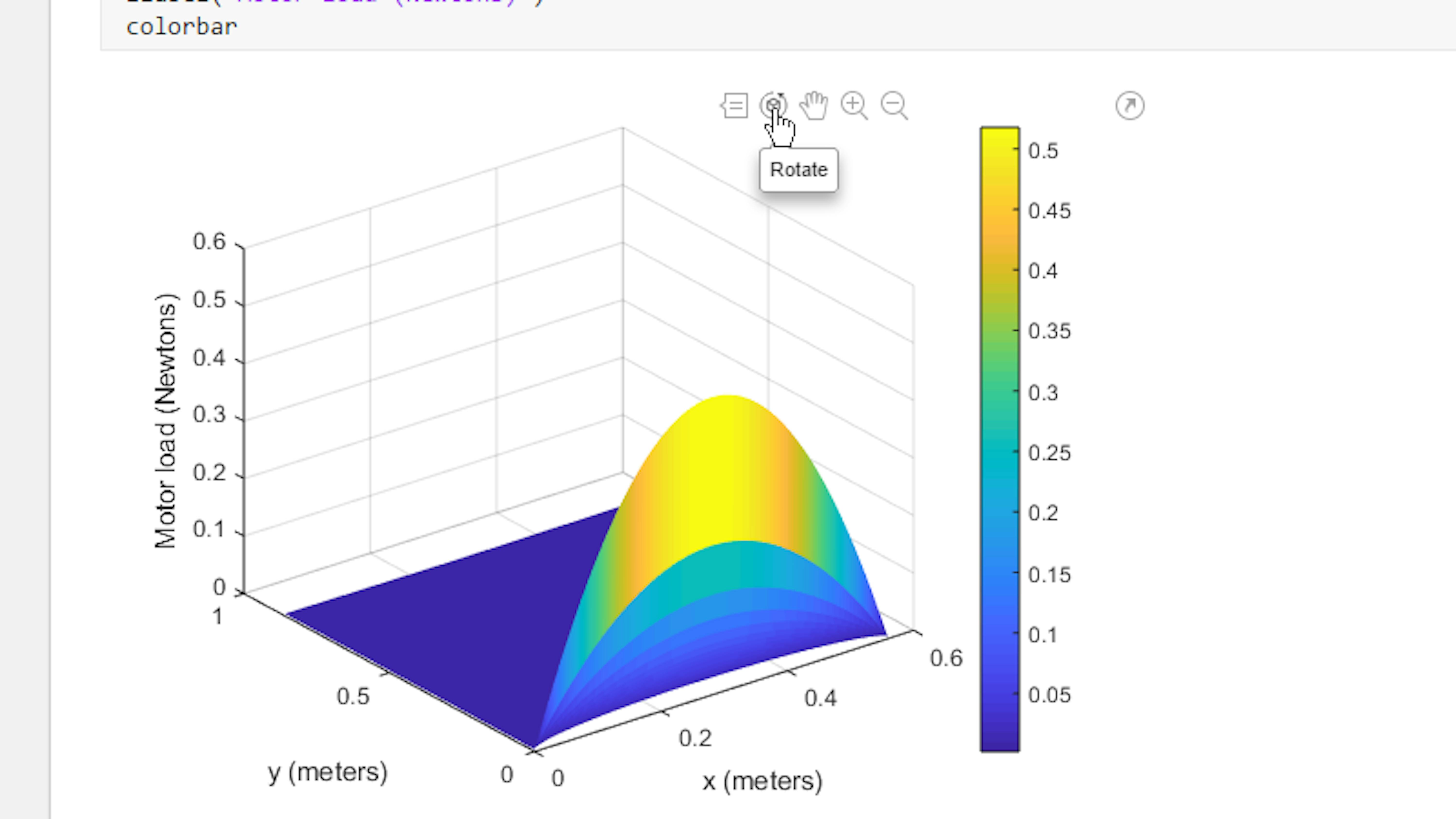
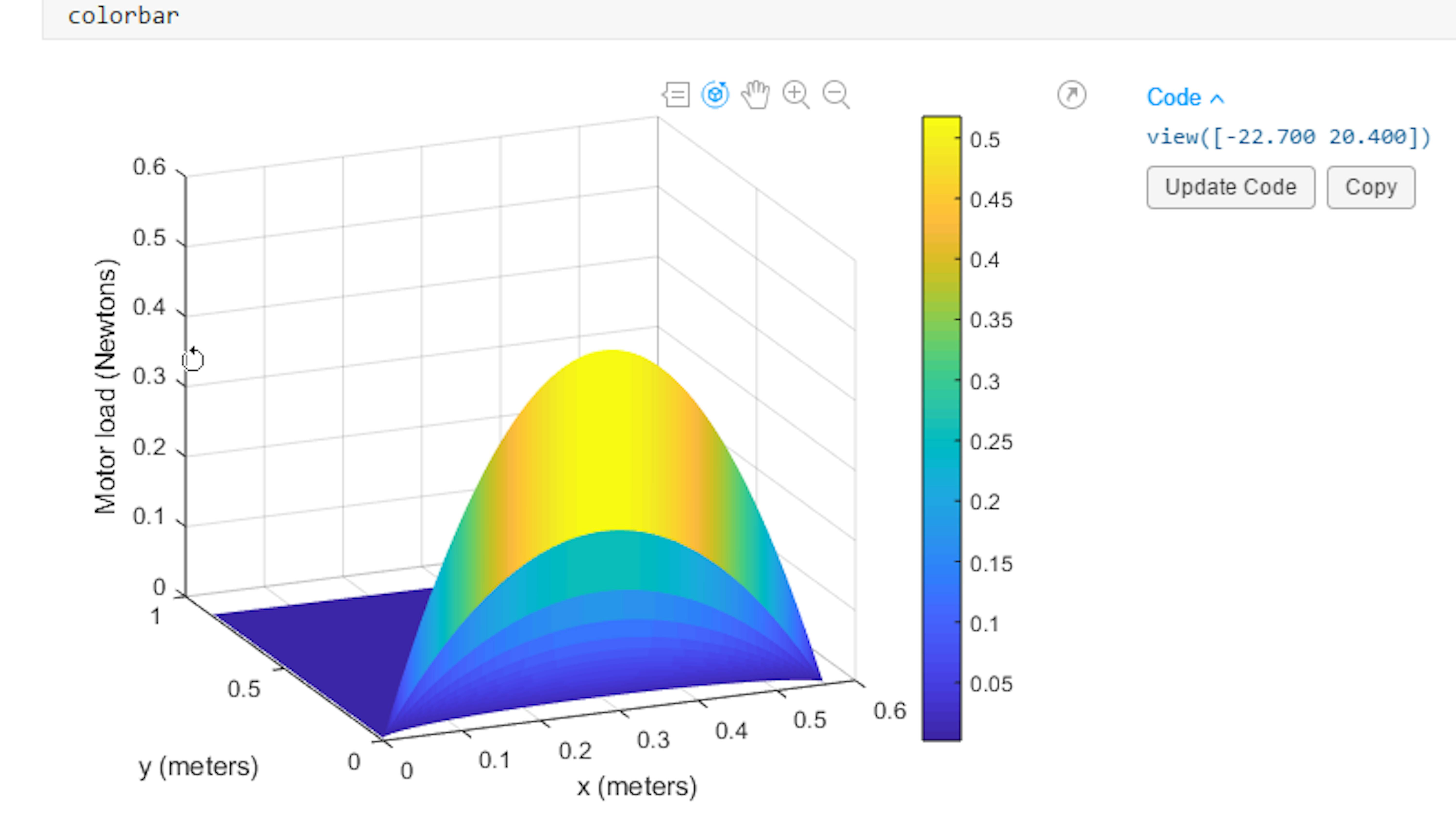
Now that the motor load Tau is defined at every position on the whiteboard, you can visualize it in MATLAB. Create a simple surface plot using the surf function in MATLAB. To do so, run the section of code in Task4.mlx under the heading Plot torque at every position.
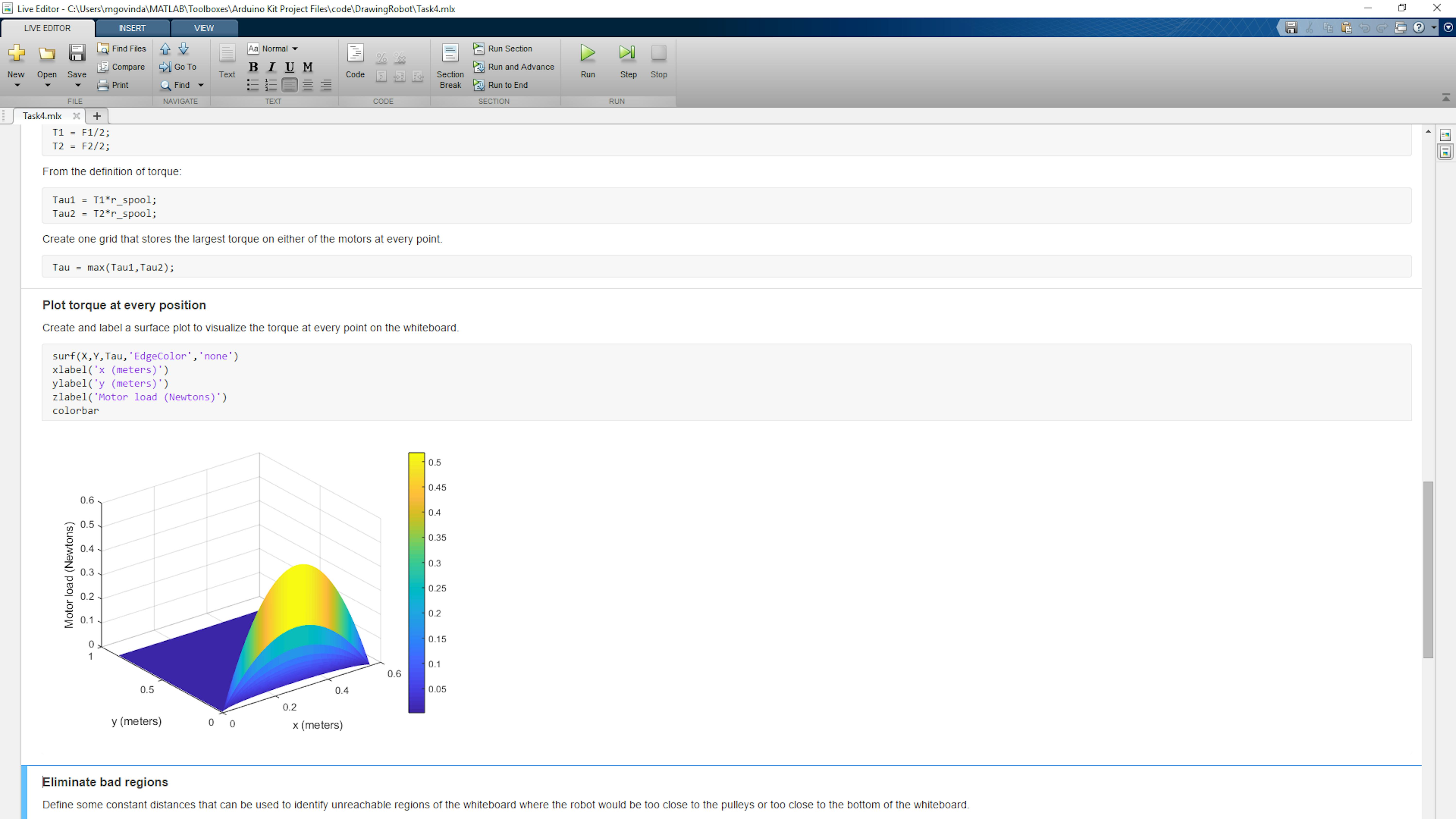
Explore this plot. Click the icon marked Rotate. Then click and drag the plot to examine the surface from all sides and get a better sense of what the torque is like at different positions on the whiteboard.
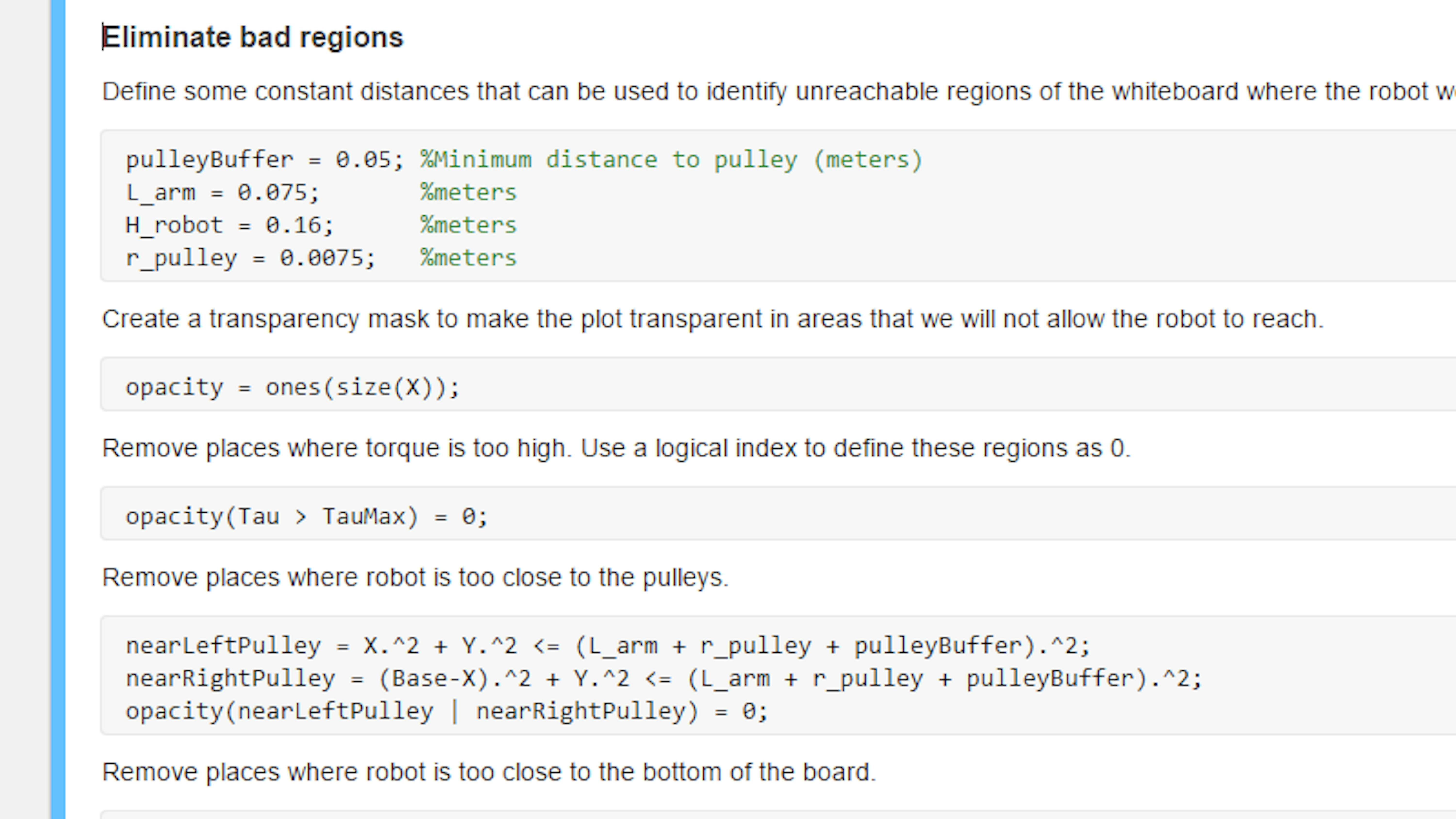
ELIMINATE BAD REGIONS AND PLOT IMAGE
Now make a plot that removes the regions the robot should not move to. This includes two types of regions. First, remove the regions where the torque is too high. Then remove the regions where the robot cannot go because it is too close to the pulleys or bottom of the whiteboard.
To "remove" these regions from our plot, we'll define a transparency mask for the plot. The plot will be visible at regions the robot can reach and transparent at regions the robot cannot reach. In MATLAB, the data that defines these regions is called AlphaData. To create the opacity variable and remove the unreachable regions, run the section of code under the heading Eliminate bad regions.
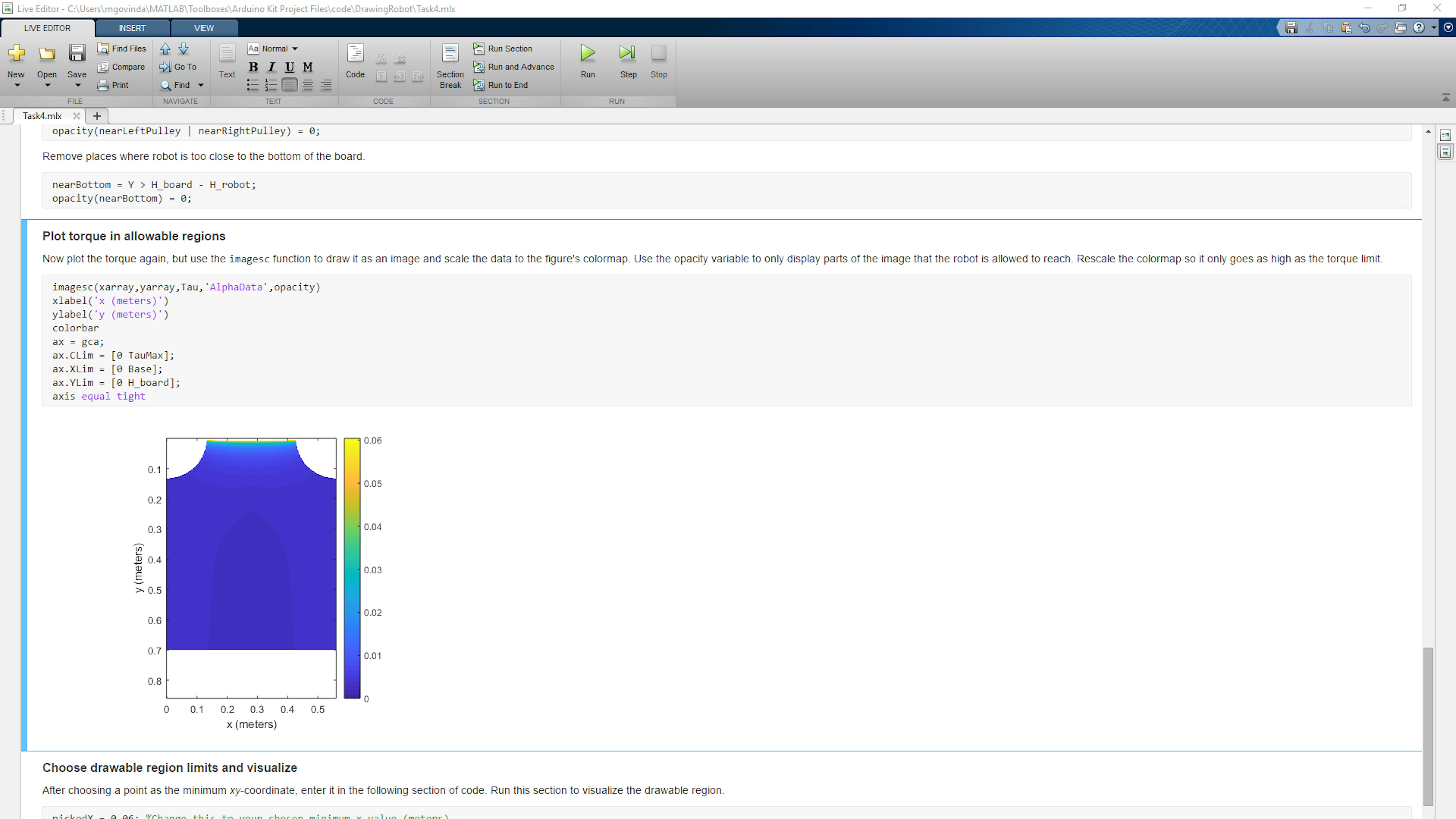
Now, you can use the opacity variable in a plot. Create an image plot to view the Tau data in 2D and include the opacity variable as the plot's AlphaData . Also, you can adjust the color limits so that they scale to the maximum value of the visible portion rather than the maximum value over all of Tau . This 2D plot will show you which parts of the whiteboard the robot can and cannot reach. The transparent areas represent those where the robot can't reach. Create this plot by running the code in the section Plot torque in allowable regions in Task4.mlx.
DEFINE AND SAVE DRAWING LIMITS FOR YOUR WHITEBOARD
Next, you'll define the part of the whiteboard that you will allow the robot to draw on. You can choose where you want the minimum x and y values to be for your drawing region. These are likely to fall somewhere along the curve that defines how close the robot can get to the left pulley. Use the Data Cursor tool in the live script to select a point and check its x - y coordinates.

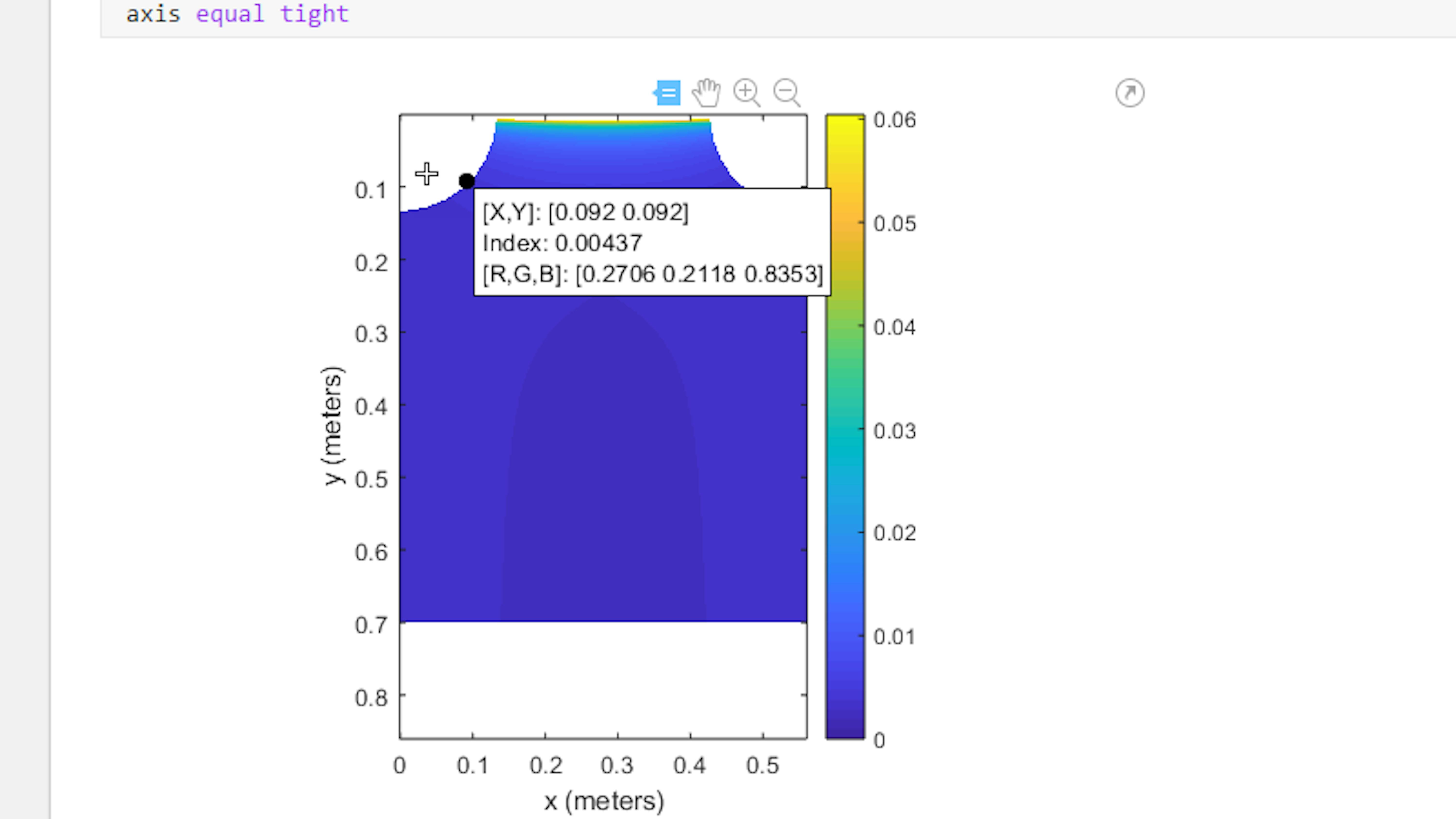
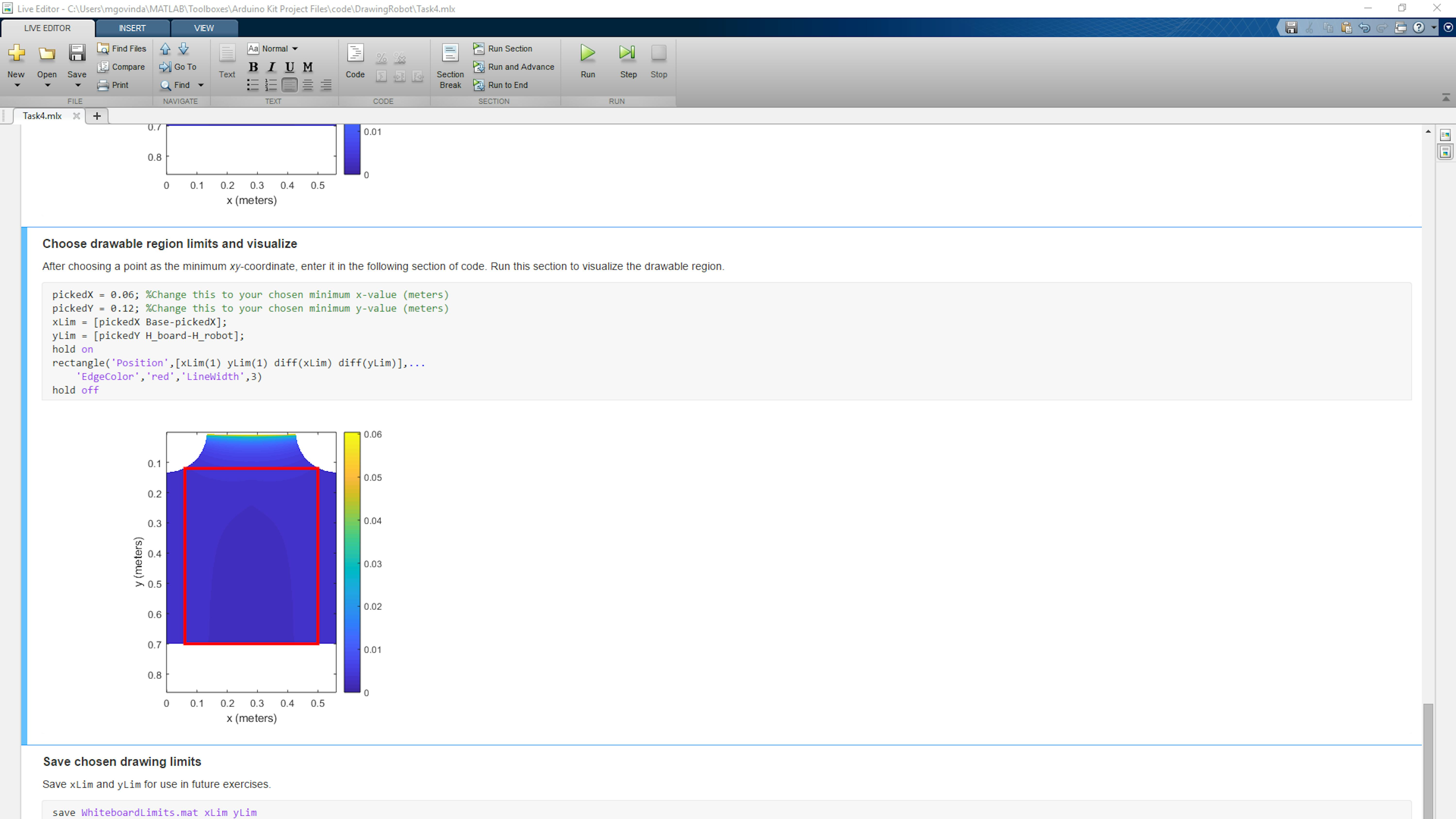
Record the x and y values from the plot in the code. Find the next section of Task4.mlx under the heading Choose drawable region limits and visualize . Replace the pickedX and pickedY variable values with the values you selected in the plot.
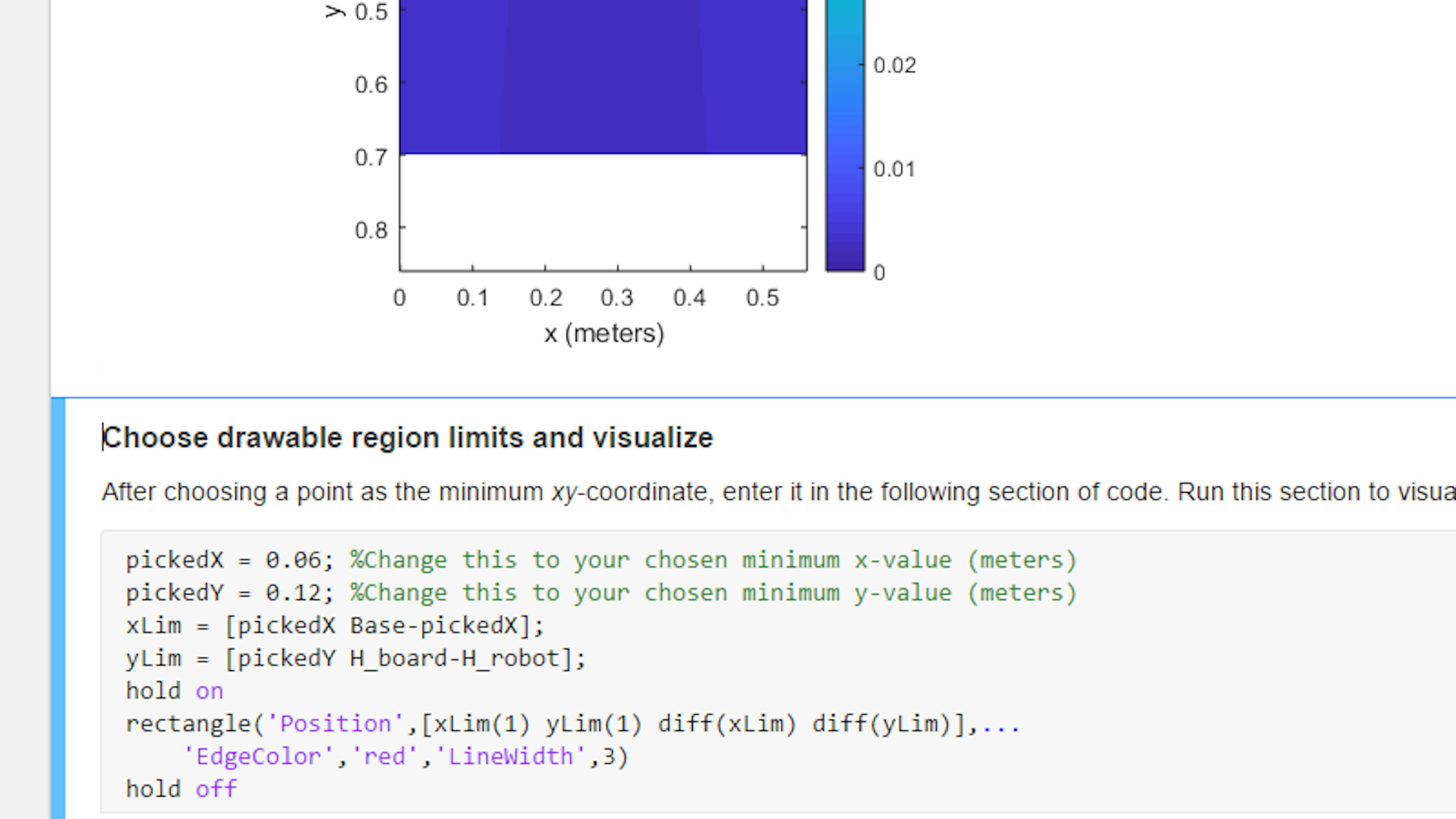
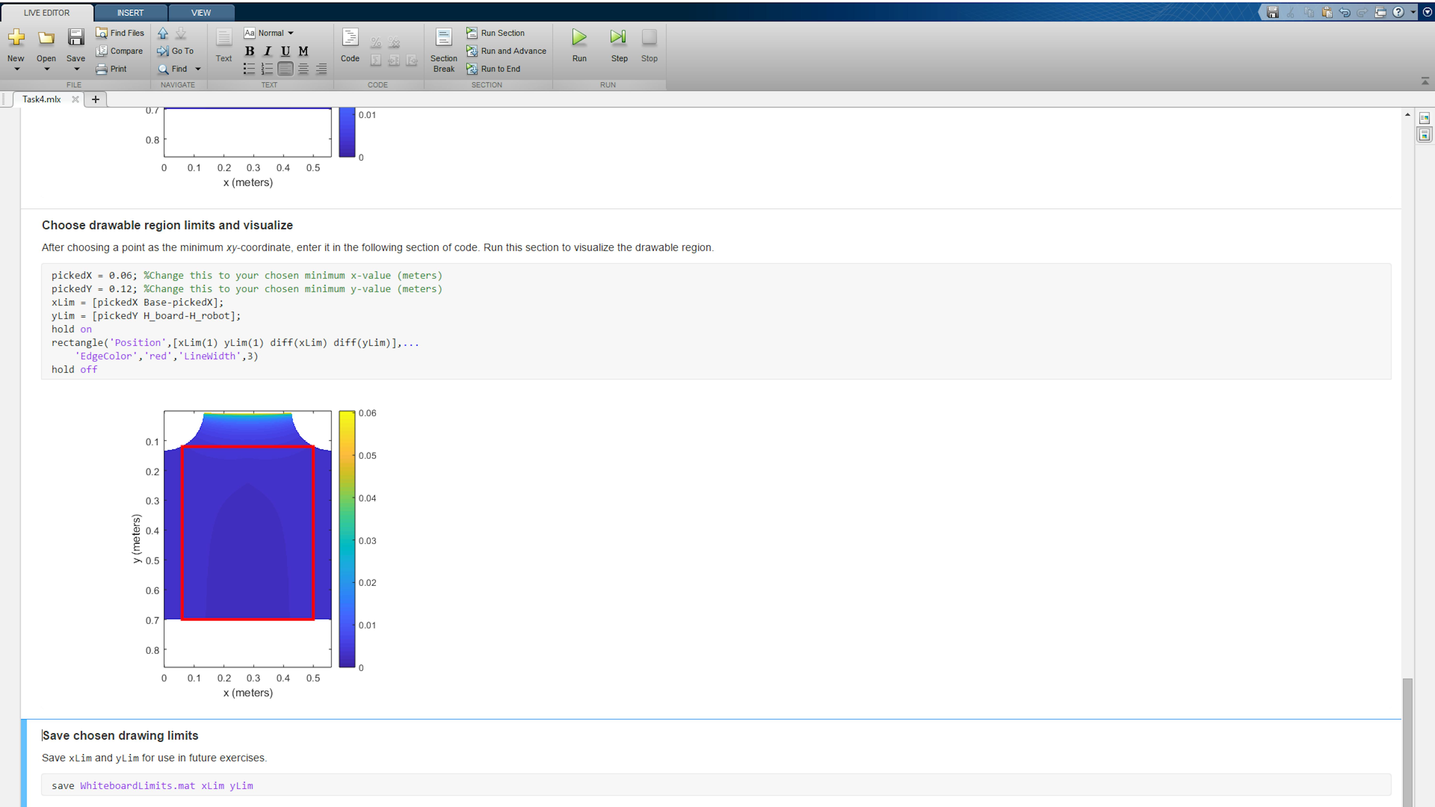
You can visualize the drawable region of the whiteboard by overlaying a rectangle on the plot you made previously. To keep the previous plot and add to it, use the hold on command. Use the rectangle function to draw the rectangle. To do this and verify that your drawable region looks correct, run the code under the heading Choose drawable region limits and visualize in Task4.mlx.
If you're happy with the size and shape of the rectangular region selected, you should store the values of xLim and yLim in a MAT-file for later use. Run the section of code under the heading Save chosen drawing limits in Task4.mlx so that you can use those values in future exercises.
FILES
- Task4.mlx
LEARN BY DOING
We created the variable Tau to contain the greatest load on either of the motors at every position on the whiteboard. Create a new variable containing Tau2 - Tau1 that describes the difference in load between the right and left motor at every point on the whiteboard. Plot this just as you plotted Tau . Where is the load greater on the right motor than the left? Where is there a smaller load on the right motor than the left?
Use the app SimplePlotterApp to drive the robot around the whiteboard as you did in an earlier exercise. Confirm what you've seen in the plots in this exercise. For a given voltage, the motors will run slower if there is greater load. Check how fast the motors run at the top of the whiteboard versus the bottom. Check how fast each motor runs at the left of the whiteboard versus the right. Does this match the plots you've created?
The size and dimensions of the drawable whiteboard region can be defined by math equations. Let's say you wanted a square region where the width and height were the same. Use the defining equations to calculate the pickedX and pickedY values that would give you a square drawable region. Enter these values in the live script Task4.mlx, and then run the script again to check the accuracy of your calculations.
EXERCISE 5:
4.5 Draw preprocessed images
Let's draw an image of something real. In this lesson, you'll load some data that stores the line traces from a real image. You'll learn how to interpret this data and build an algorithm that tells the robot to draw each line segment and then raise the marker and move to the next line segment. You'll learn how to scale the size of the line drawing so that it fills up the drawable space on your whiteboard. Finally, you'll create one MATLAB function that can perform all these steps.
In this exercise, you will learn to:
- Plot image data in MATLAB
- Loop through and manipulate data in a cell array
- Convert data from pixels to physical distances
- Design an algorithm to draw an image in multiple segments using a loop
UNDERSTANDING HOW TO READ IMAGES IN MATLAB
MATLAB can work with images in common image file formats. The general workflow is first to read the image into a MATLAB variable. Then you can apply functions to change the image or visualize it, and you can write the image to a new file.
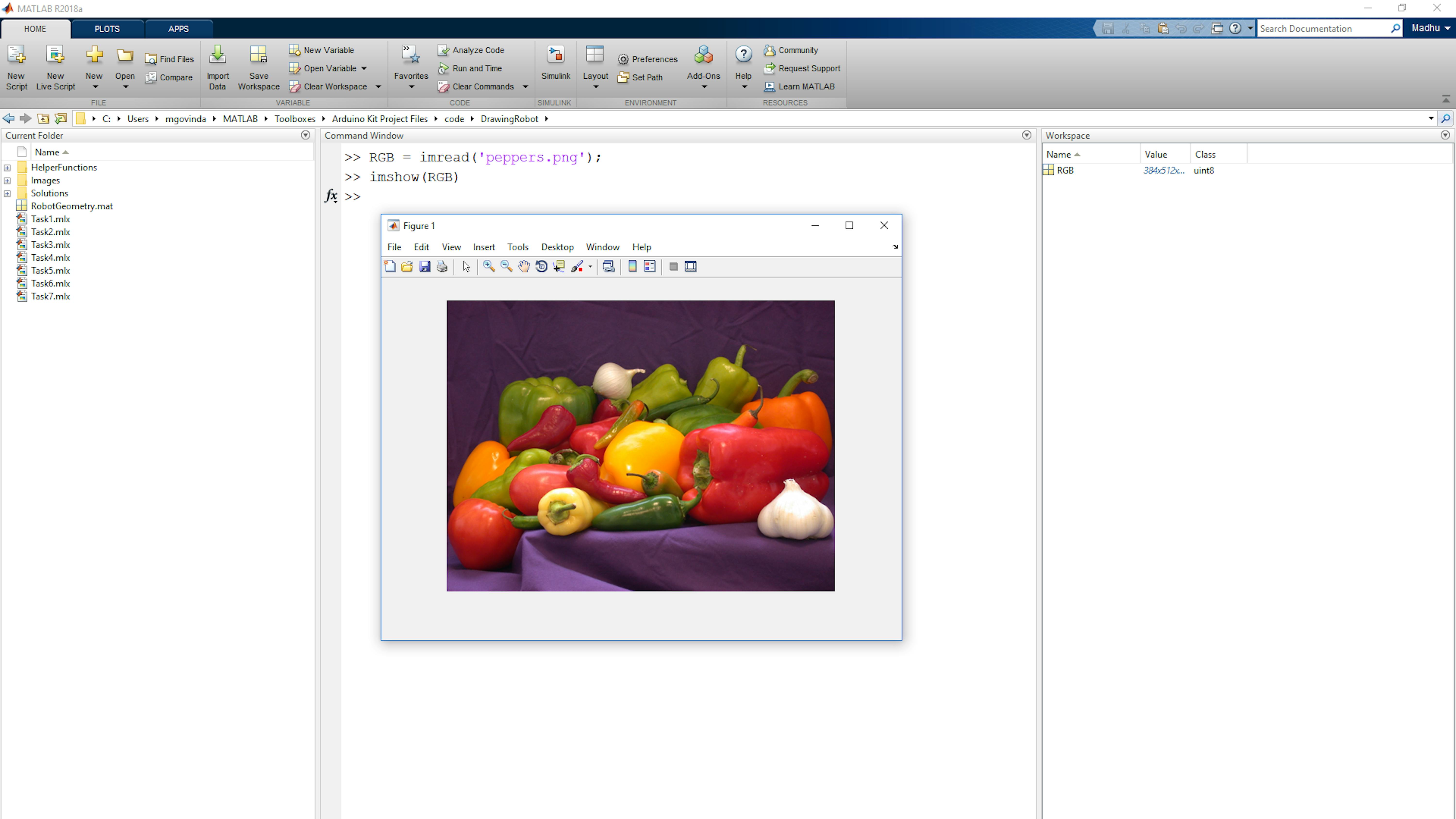
To read an image into MATLAB, use the imread function. An image that ships with MATLAB is in the file peppers.png. Read this by entering the following at the MATLAB command line.
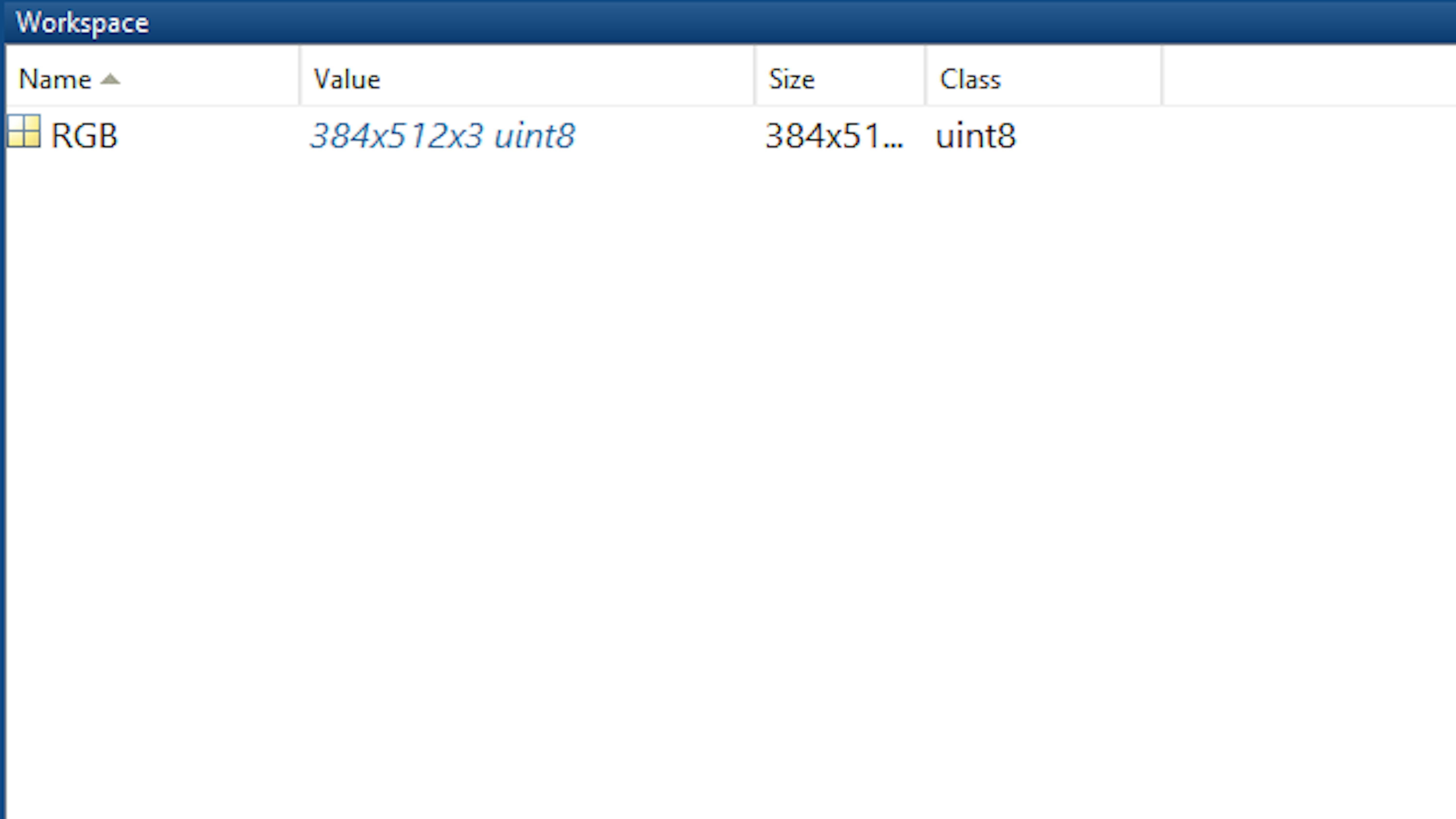
>> RGB = imread('peppers.png');Examine the RGB variable in your Workspace. Note that the variable is three-dimensional and of type uint8. Each one of the components (R, G, B) representing one of the basic colors gets 8 bits to store its value in digital form. This means that you can work with images of 24-bit color depth (8 bits or 1 byte for each one of them).
View the image using the imshow function. Execute the following statement at the command prompt.
>> imshow(RGB)
The three components of the variable represent the red (R), green (G), and blue (B) information of the image respectively. You can imagine this as three grids of numbers stacked on top of each other, one for each color plane. To get a sense of what this means, you can visualize just one plane of the image. To see a representation of the red plane data, use the following command to view the image regions that have the most red:
>> imshow(RGB(:,:,1))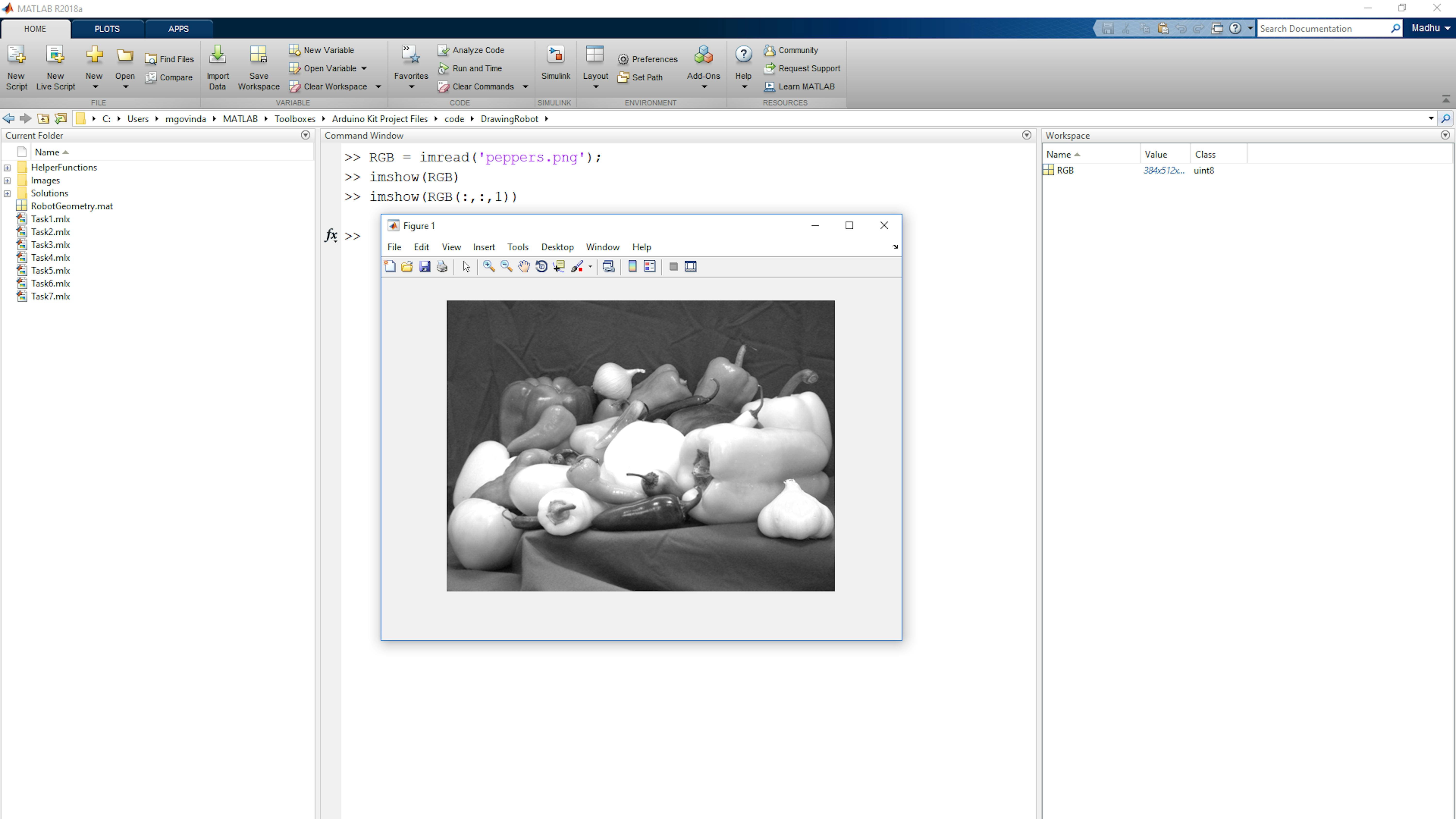
Note how representing a single color plane of an image results in a greyscale image. This can be confusing. Alternatively, you can view an image in MATLAB without even loading it into a variable simply by calling imshow on the file itself. Run the following command to do this with the peppers image.
The result is the same as when we displayed the full color matrix.
>> imshow('peppers.png')The result is the same as when we displayed the full color matrix.
PLOT AN IMAGE OF A DRAWING TO REPLICATE
The robot is not able of drawing full RGB planes, and not even greyscale images. The current design needs vector graphics as an input. This means that whatever image you want to draw will need to go through some image processing first to turn it into the proper form.
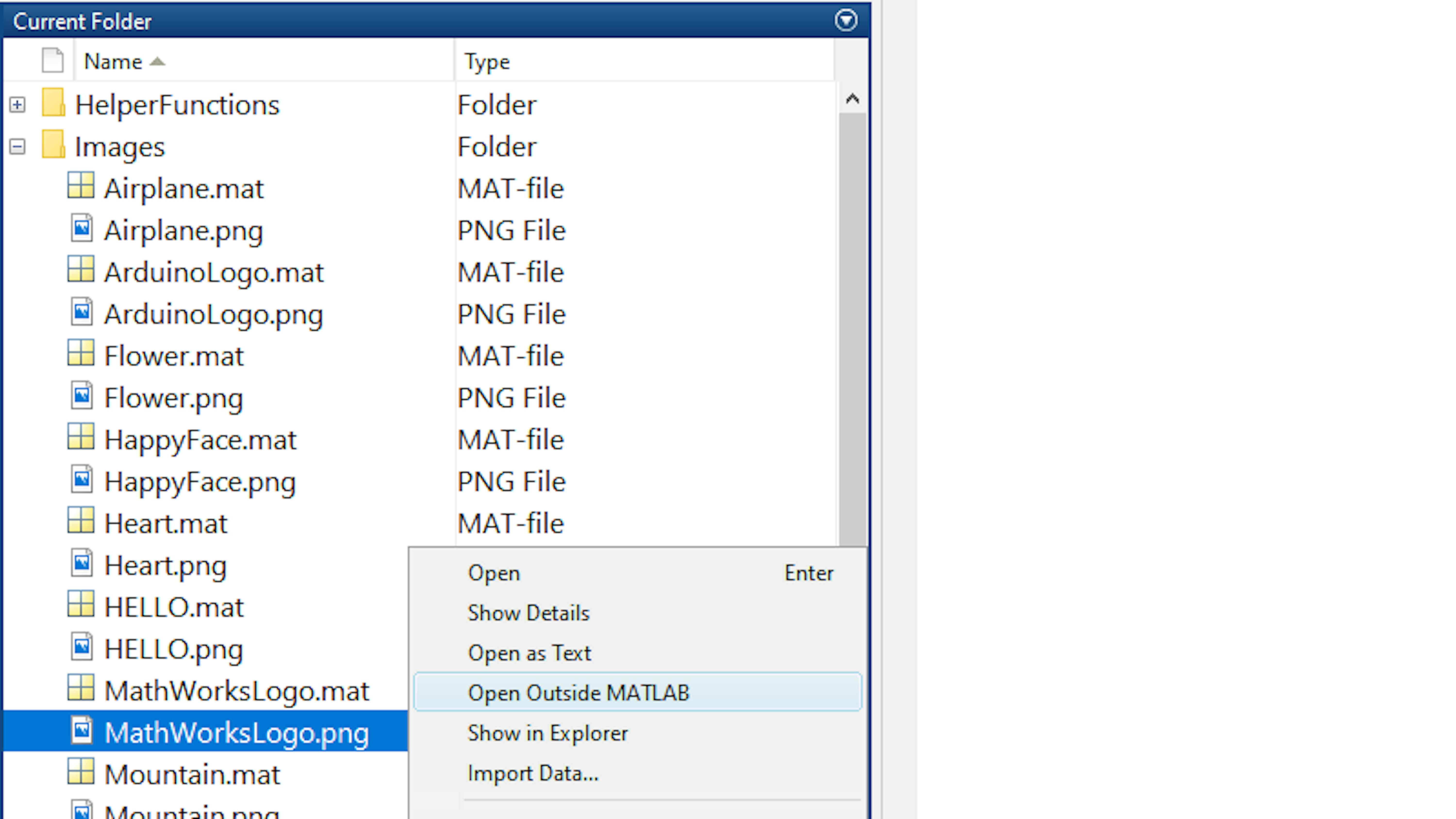
A few sample line drawings have been processed into a drawable form and provided for you. (In the next exercise, you'll learn how to generate these yourself). The Images folder contains both the original images and their corresponding MAT-files containing the path to draw. Find the file MathWorksLogo.jpg. Right click it in the Current Folder and select Open Outside MATLAB to see what it looks like in your system’s image viewer. Note that different operating systems have different image viewers.
Next step is checking whether the processed file looks similar to the original image. For that you will open the live script Task5.mlx :
>> edit Task5And run the code in the Plot sample image section to see this image plotted in MATLAB.
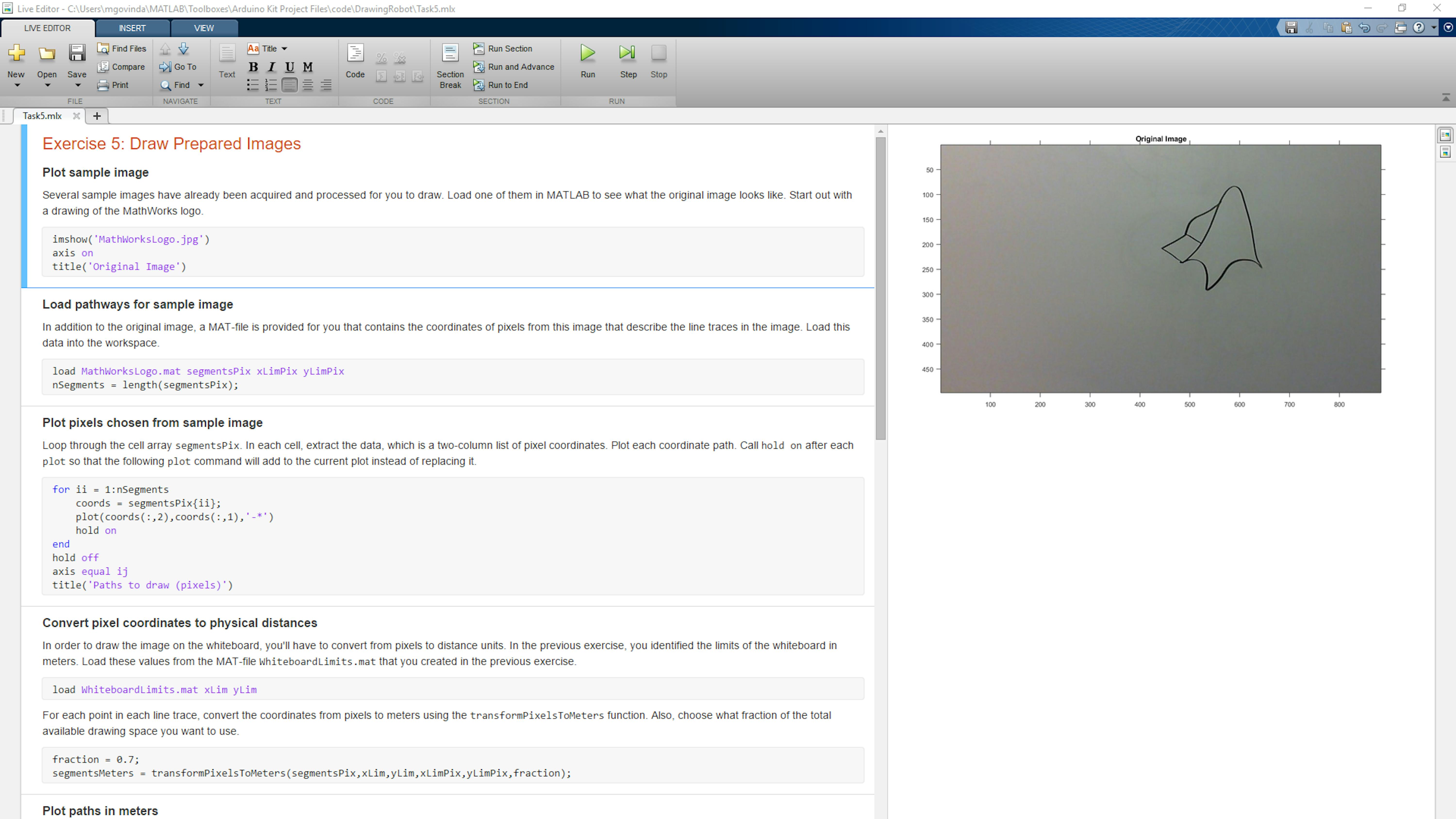
As you can see, the outcome of the plot is a vectorized version of the original image. This kind of image can easily be translated into motor movements. Follows the process on how to reach this kind of image from any image you may have as point of departure. But first, we need to build the understanding of some basic tools within MATLAB that will let you perform the needed operations.
UNDERSTAND CELL ARRAYS IN MATLAB
So far you have been working with different types of variables in MATLAB. You have created objects to represent the Arduino device and its components. You have created numeric scalars and vectors to store numeric values. And you have looked at 3-dimensional uint8 data that represents images.
Sometimes it is useful to combine multiple pieces of data into a single variable. It can be useful for grouping data of different sizes or types. To do this, you can use a data container called a cell array. There are many different reasons cell arrays can be useful, but for the purposes of this exercise, we'll focus on using them to store numeric arrays of different sizes.
To see how cell arrays work, first create some numeric arrays of different sizes. Run the following code at the MATLAB Command Prompt to create three different magic squares.
>> a = magic(3)

>> b = magic(4)

>> c = magic(5)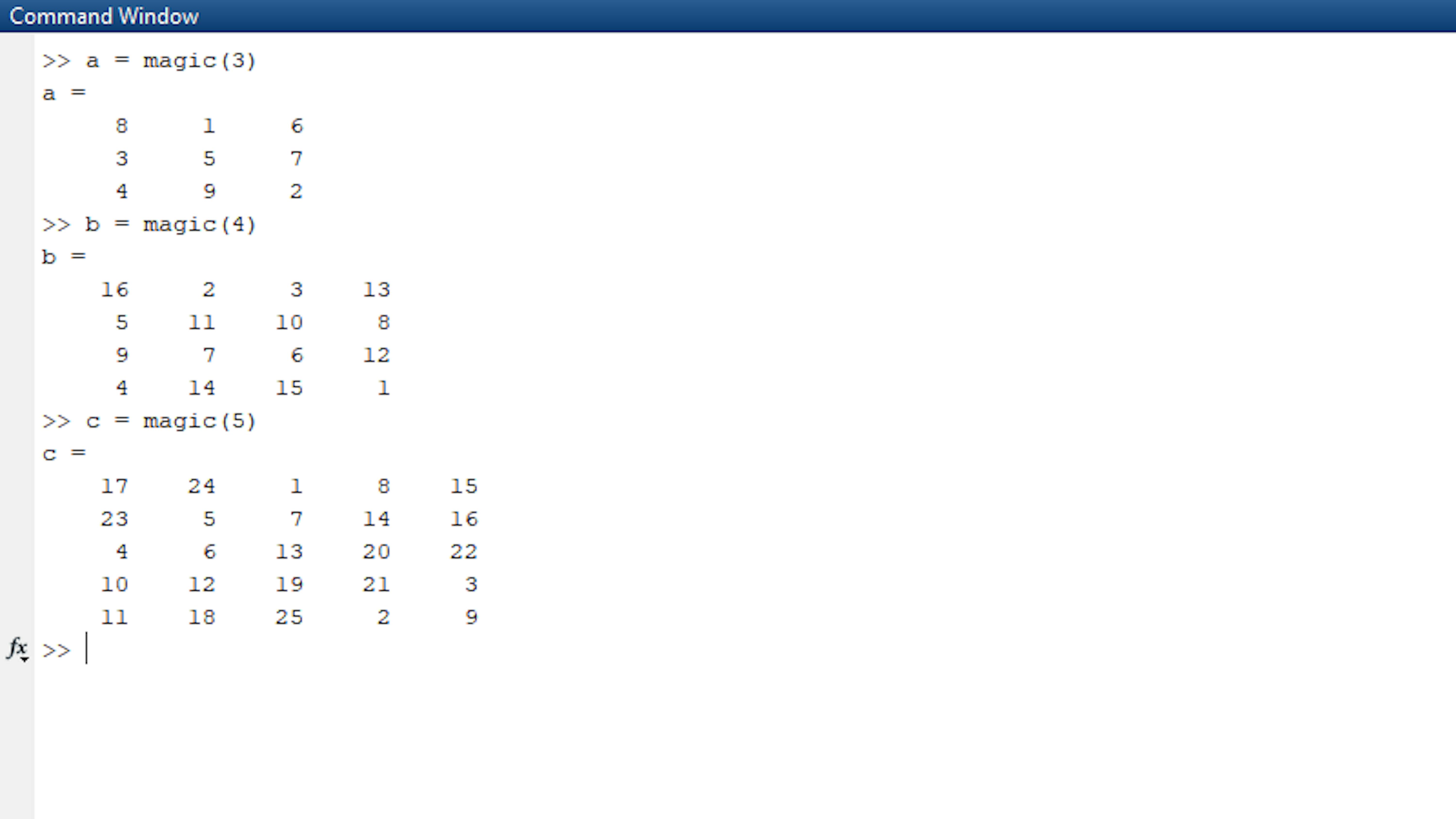
Note that the resulting arrays each have different dimensions. Now, create a single variable that stores the data from a , b , and c in the first, second, and third elements respectively. To do this, use a cell array. Note that you use curly braces {} to construct cell arrays. Run the following code:
>> C = {a b c}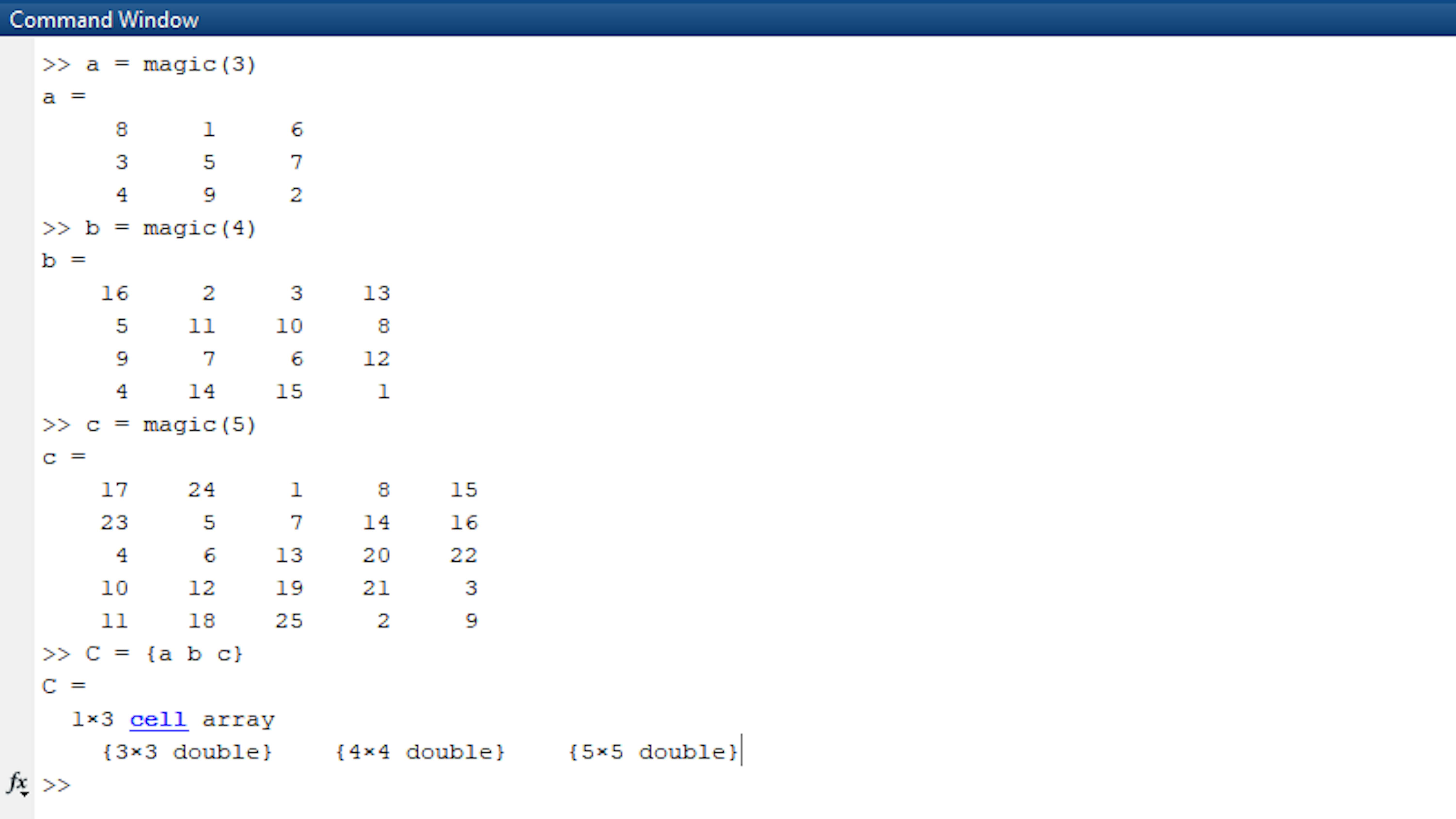
The cell array C (capitalized) has size 1x3, but each element contains a numeric array. Reaching inside a cell array to pull data out of a variable is called indexing. With a numeric array, you use parentheses () to pull out the numeric elements. With a cell array, if you use parentheses, you'll pull out the cell elements. Compare the output of the following two statements:
>> a(1,1)

>> C(1,1)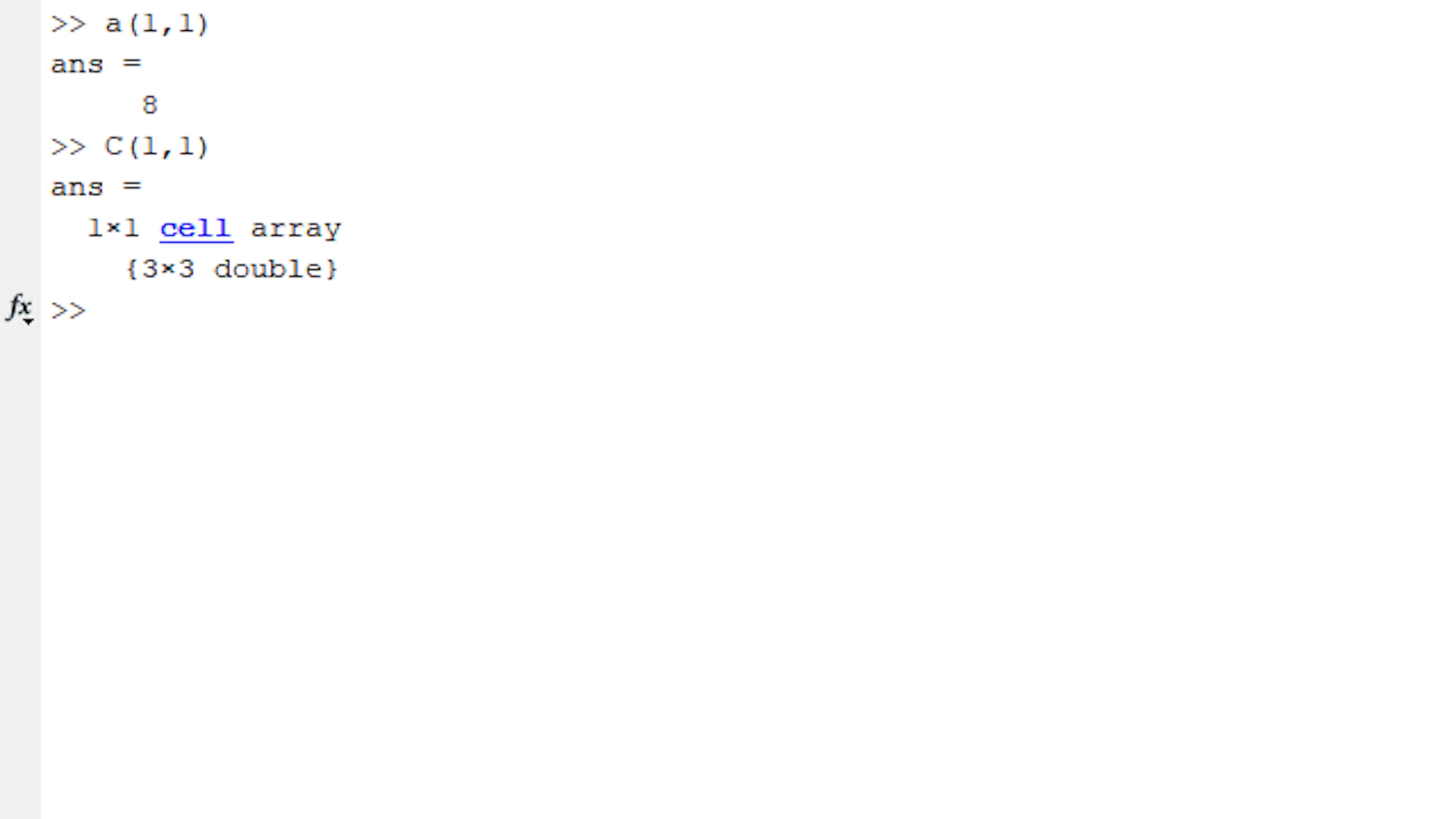
The call to C(1,1) returned a link to the object, which is the array a, but did not display the content in it. If you want to reach inside a cell array to pull out the data it contains, you will have to index with curly braces {} . To get at the data contained inside the cell C(1,1) , execute the following:
>> C{1,1}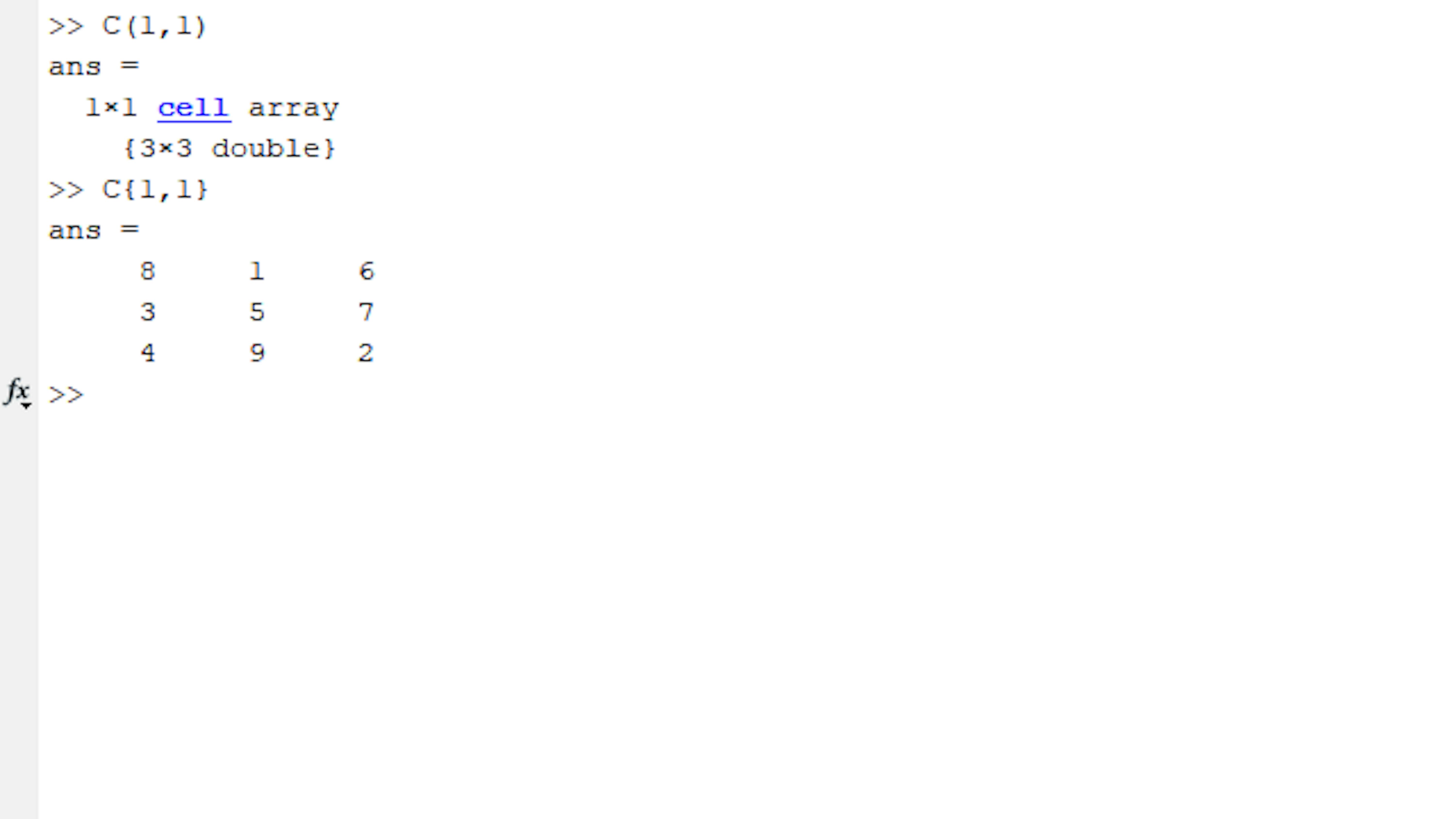
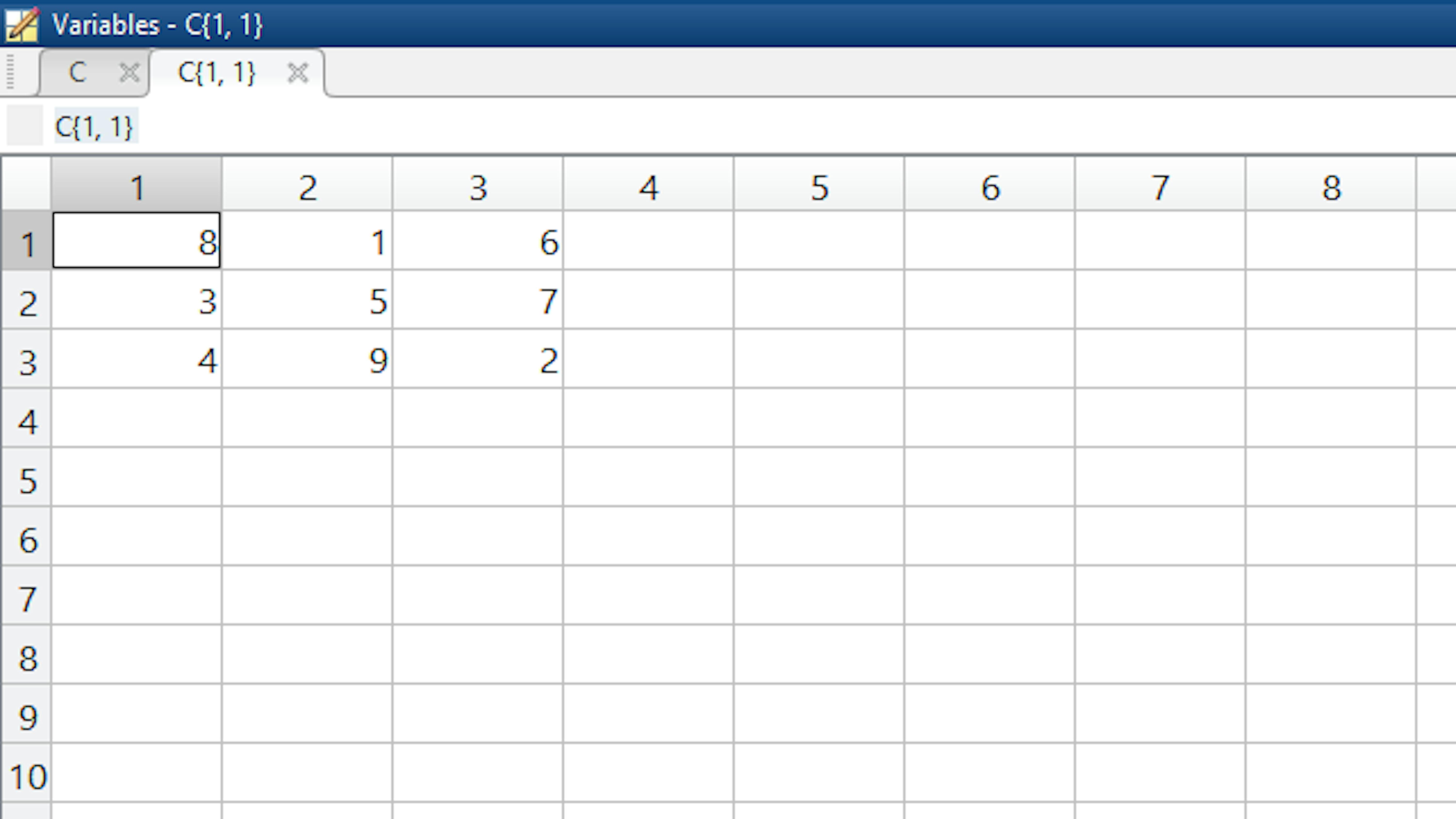
You can also examine the contents of a cell array by double-clicking it in the Workspace. This action will bring the contents up in the Variable Editor.
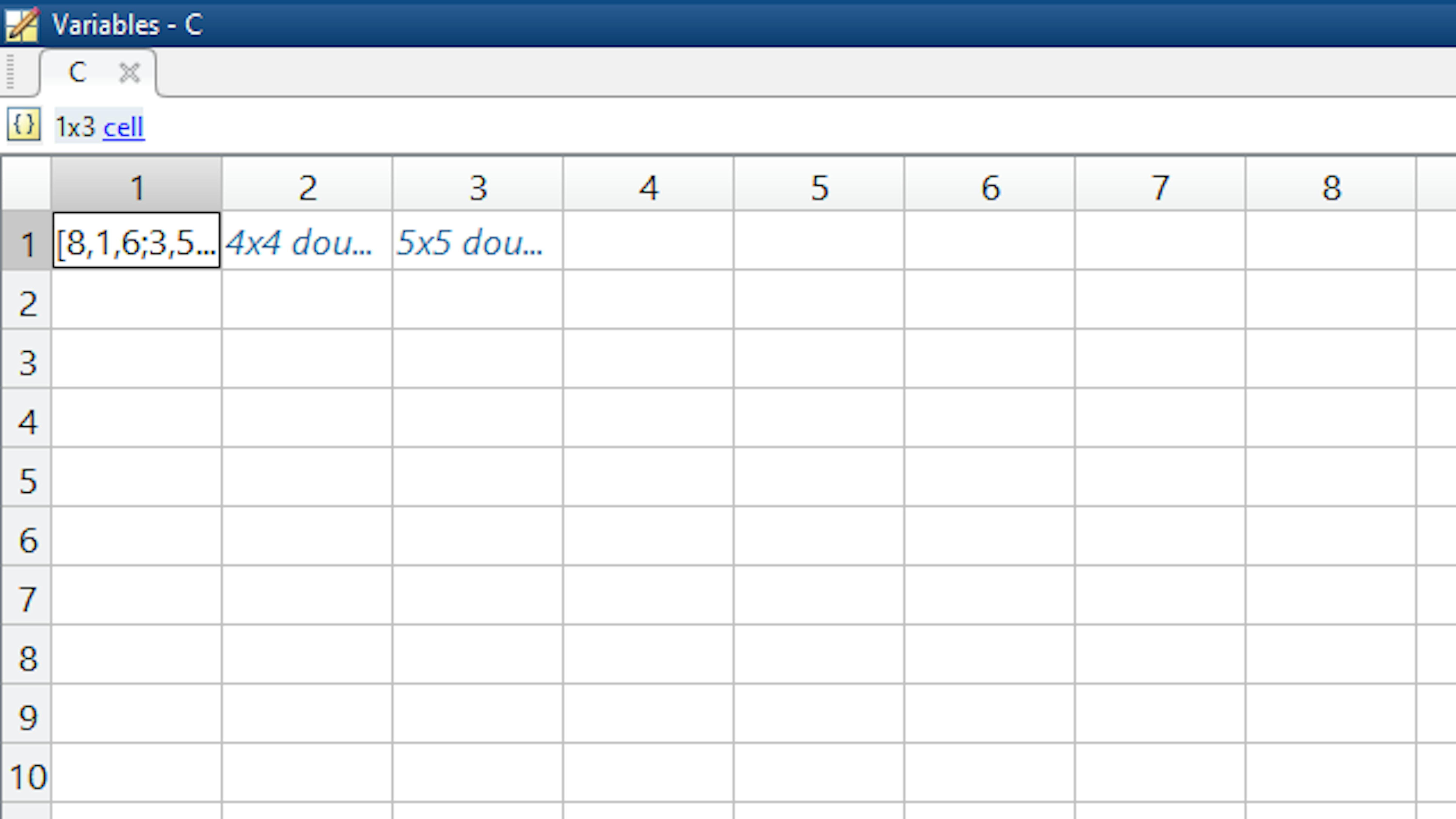
Double-click a cell to dig in and view the contents of that cell, in a separate tab.
You will use cell arrays in the following sections because they allow you to store coordinate lists of different sizes in a single MATLAB variable. We will work in this way to keep our code tidy. Remember that it is good practice to have your code made in a way that is easy to read by others.
LOAD AND PLOT COORDINATES FOR AN EXISTING IMAGE
The coordinates of the points to plot are stored in a cell array. Run the section Load pathways for sample image in Task5.mlx to bring the data into MATLAB.

Double-click the segmentsPix variable in Workspace to open it in the Variable Editor. Notice that it is a cell array with three elements, each of which contains a two-column array of doubles with different number of rows each.
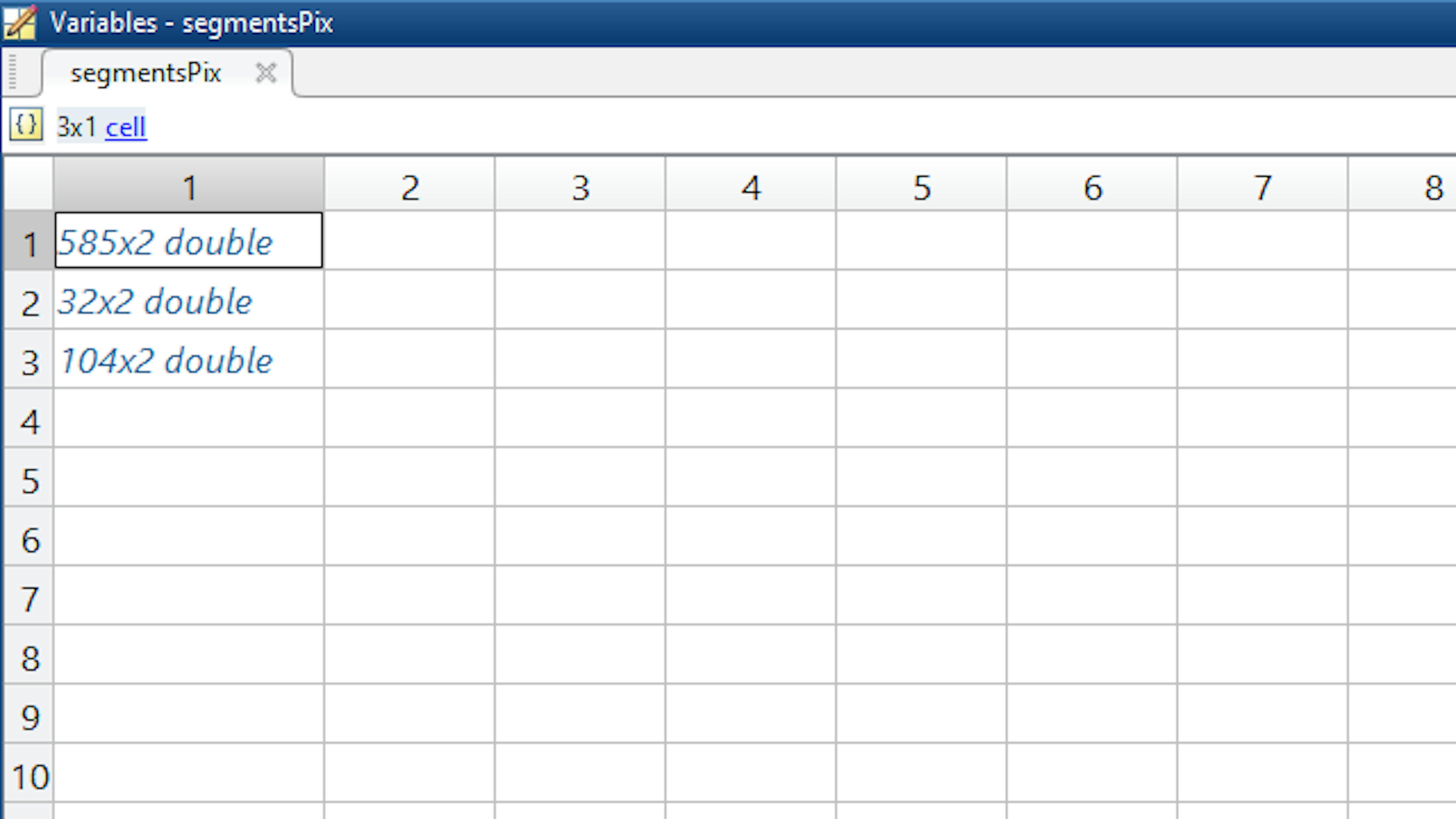
In other words, there are three different line traces in this image file. Double-click one of these elements to see the data contained in that cell. These values represent the pixel coordinates in the image for the selected line trace.
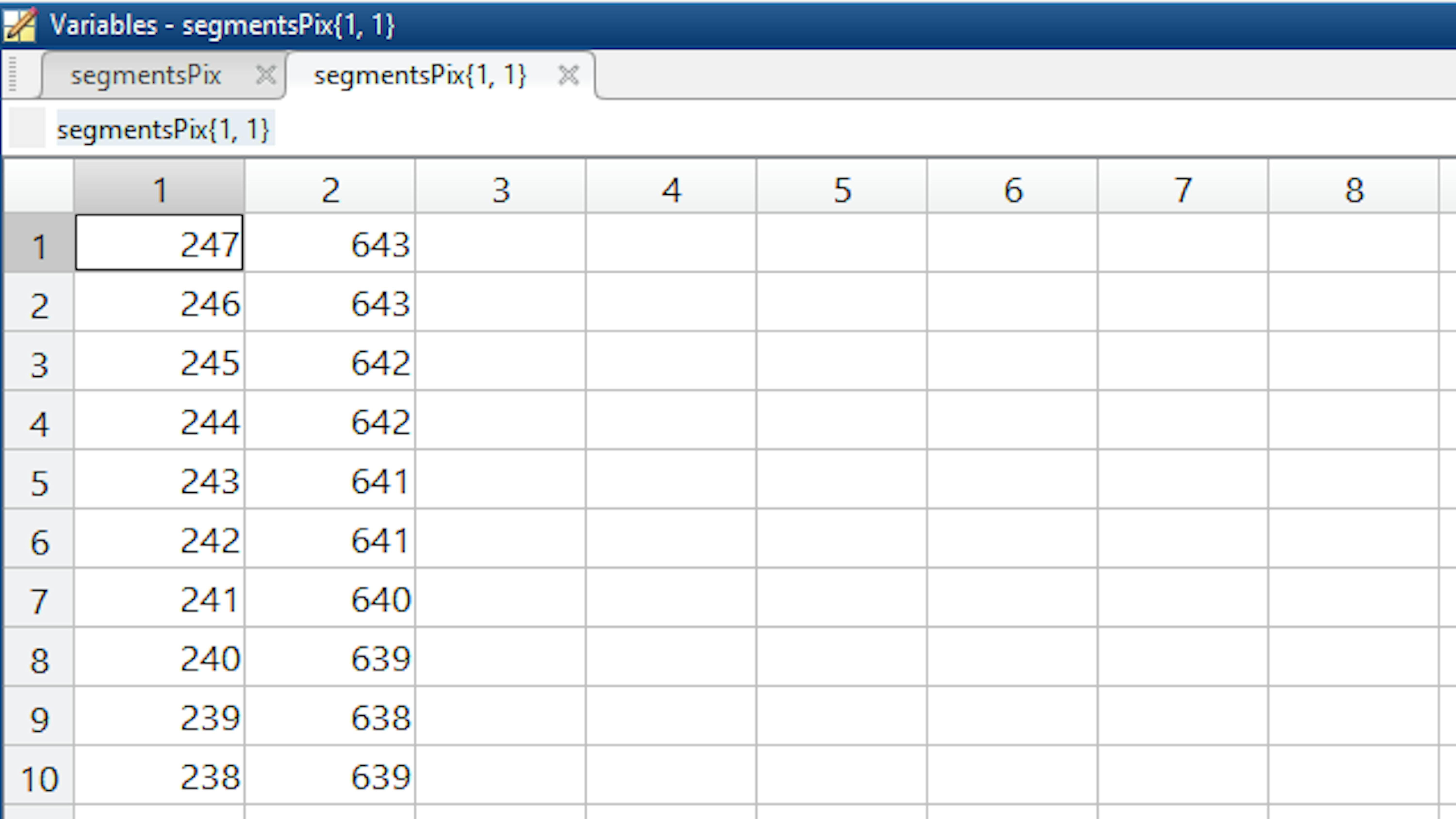
The nth element of the segmentsPix cell array variable can be accessed using curly braces, as in the following command.
>> data = segmentsPix{n};
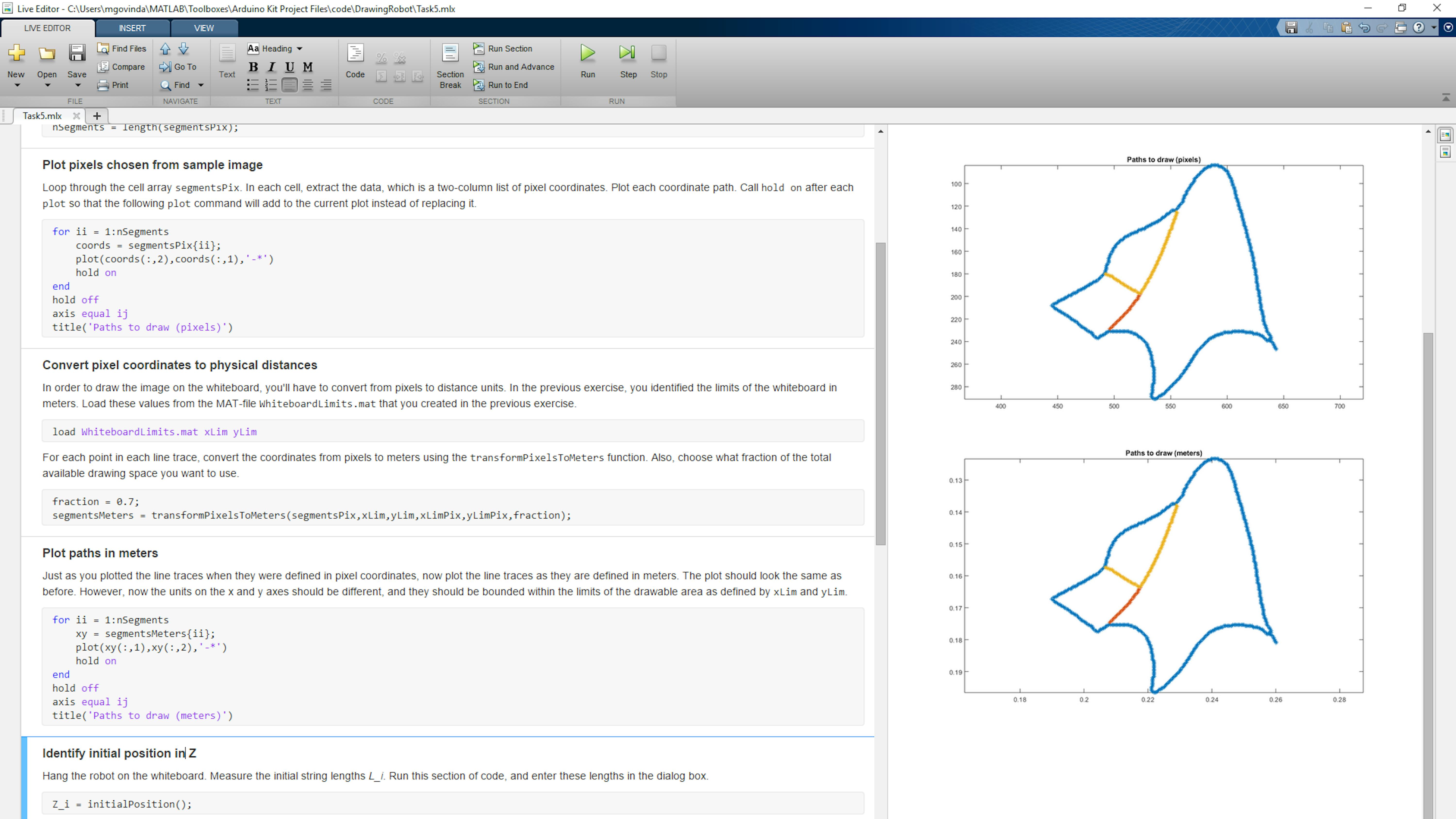
Find the section in Task5.mlx under the heading Plot pixels chosen from sample image. Note that this section of code contains a for loop with loop index ii . In each iteration of the loop, the iith element of segmentsPix is extracted and plotted. Run this section to see the pathways stored in this variable.
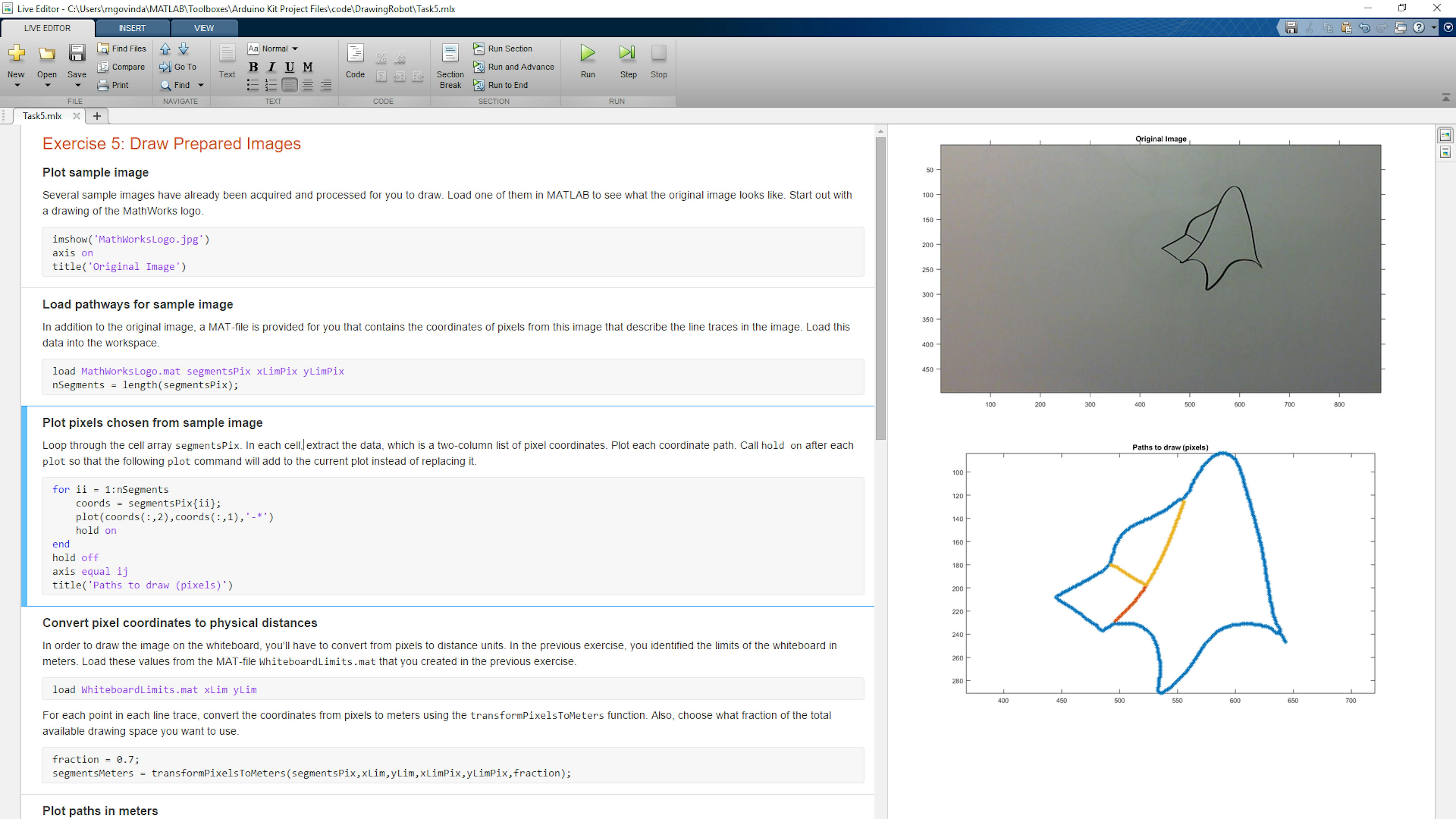
As you can see in the image, the different pathways are drawn in different colors. When we design our own algorithm, we will have a similar result to whatever image we capture: there will be different pathways that, when joined together, will represent the full image.
UNDERSTAND SCALING TO PHYSICAL UNITS
To decide where to draw an image on the whiteboard, you will have to convert the data from pixels to metric units (meters). The whiteboard dimensions will determine the maximum and minimum whiteboard positions in meters. These values are stored in variables that we will label as xLim and yLim for x and y respectively. There will be two limits in the x axis, and two in the y axis (a maximum and minimum position for moving on each one of the axis). We define the xRange and yRange as the difference between these maximum and minimum values as shown in the following diagram.
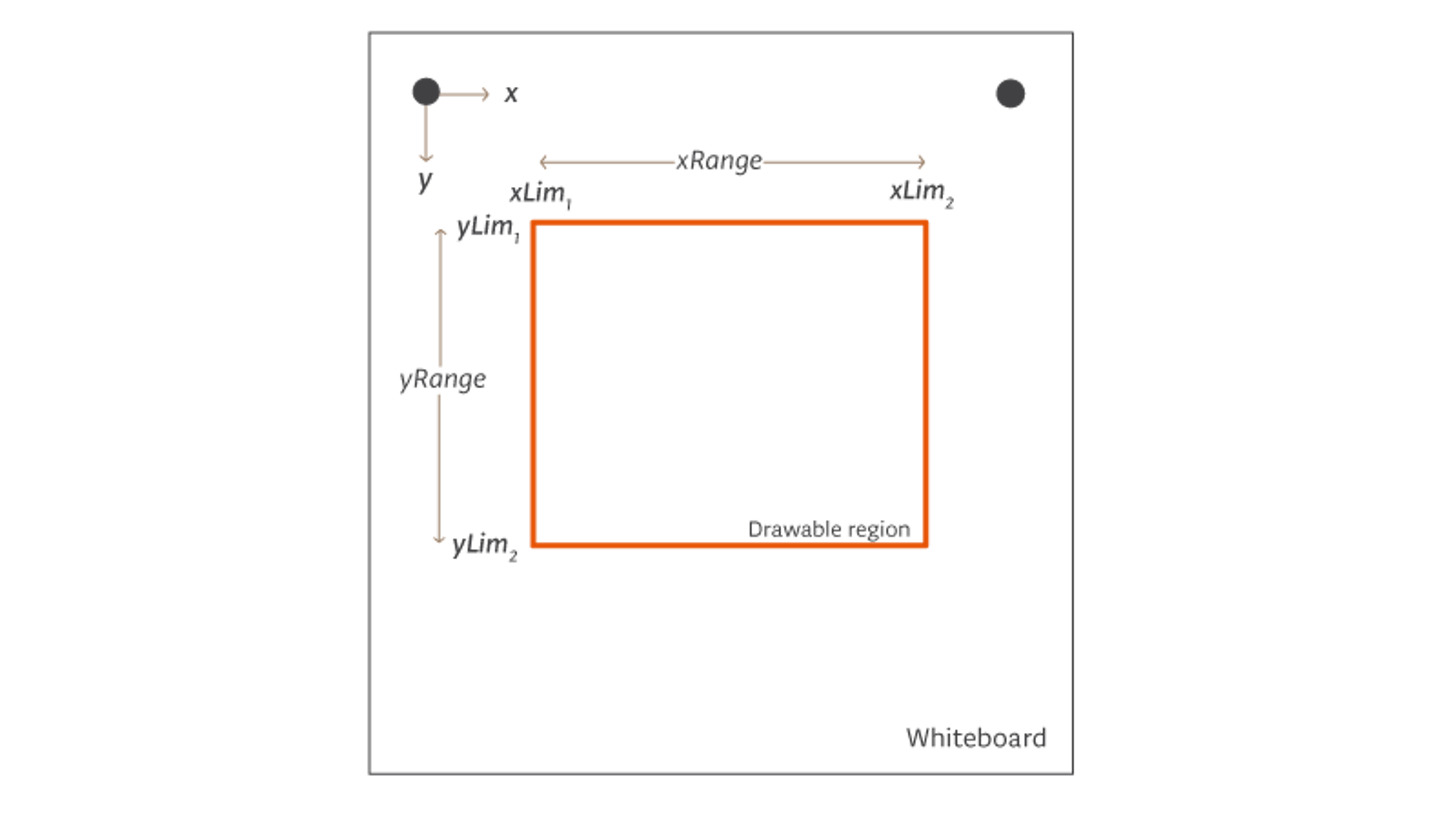
In a similar way, when looking at the image on the screen, where we count distances in pixels, the maximum and minimum pixel positions in x and y for the image we want to draw are stored in the xLimPix and yLimPix variables. We define the xRangePix and yRangePix as the difference between these maximum and minimum values as shown in the following diagram.

It seems obvious that to convert from pixels to distances, you'll need to multiply the pixel values by some scaling factor. That scaling factor will be one of the following two quantities:
${xScaleFactor}=\frac{{xRange}}{{xRangePix}}$
${yScaleFactor}=\frac{{yRange}}{{yRangePix}}$
As we have a bi-dimensional image, and the drawing surface is not connected by-design to the image size, we will end up with two different values: one corresponding to the translation of the image to the board looking at the x axis, and another one for the y axis. We need to decide for one of the two possible scaling factors. The choice of which scaling factor to use depends on which one is smaller. This will be related to the aspect ratio of the whiteboard drawing area versus the image to draw. Consider a relatively square drawing area and a short, wide image. In this case, you would want to use the x scaling factor, as shown in the following diagram:

If the image is tall and narrow, you would be limited by the height of the image and would want to scale it by the y scale factor, as shown in the following diagram:
In other words, your algorithm will have to decide how to best convert the image from pixels to meters. The approach presented here scales the image to fill in as much of the drawable area as possible without distorting the image. But distortion is something that you should consider at a later stage, especially if your drawing area is large.
UNDERSTAND THE TRANSFORMPIXELSTOMETERS FUNCTION, LINE BY LINE
The following function converts pixels into meters. As you read through it, note how it decides which scaling factor to use, how it centers the image in the middle of the drawing area, and how it converts the measurements of each trace, translating them to the new coordinate system.
The function also allows the user to specify what percent of the available space should be used to draw the image. This is specified by the fraction input argument.
This function computes the scale factor for converting pixels to meters, then converts all the segments
in segmentsPix to meters.


function segmentsMeters = transformPixelsToMeters(segmentsPix,xLim,yLim,xLimPix,yLimPix,fraction)
First, create variables to represent the ranges xRange, yRange, xRangePix, and yRangePix.
xMinM = xLim(1);
yMinM = yLim(1);
xRangeM = diff(xLim);
yRangeM = diff(yLim);
% Determine the range of the coordinates to draw
xMinPix = xLimPix(1);
yMinPix = yLimPix(1);
xRangePix = diff(xLimPix);
yRangePix = diff(yLimPix);Calculate the two possible scale factors. The fraction factor indicates what percentage of the available
space should be used.
% Scale from pixels to real world units (meters)
xScaleFactor = fraction*xRangeM/xRangePix;
yScaleFactor = fraction*yRangeM/xRangePix;Choose the smaller of the two scale factors.
% Pick the smaller scale factor. If both are NaN, pick
0.
pix2M = min(xScaleFactor,yScaleFactor);
if isnan(pix2M)
pix2M = 0;
endBased on the chosen scaling factor and range values, identify the new origin for the scaled drawing
so that the full drawing will be centered at the center of the drawable area.
% Identify origin position of scaled drawing
centerMeters = [xMinM yMinM] + [xRangeM yRangeM]/2;
drawingOriginM = centerMeters - pix2M*[xRangePix yRangePix]/2;Loop through all segments and transform pixel values to meters for all coordinates.
Subtract the pixel origin, multiply by the scaling factor, and add the drawing origin.
segmentsMeters = cell(size(segmentsPix));
nSegments = length(segmentsPix);
for ii = 1:nSegments
% Scale all segments by the computed scaling factor
coordsPix = segmentsPix{ii};
coordsPix = fliplr(coordsPix); %Convert from row,col to x,y
coordsMeters = pix2M*(coordsPix-[xMinPix yMinPix]) + drawingOriginM;
segmentsMeters{ii} = coordsMeters;
endCONVERT PIXELS TO PHYSICAL DISTANCES AND PLOT
Now that you know how it works, you can put the transformPixelsToMeters function to use on the data you loaded from the sample image. You'll use the whiteboard x-limits and y-limits that you determined in the previous exercise. Then, for each segment, you'll convert the pixels from that segment to meters and store the new segment data in a cell array variable called segmentsMeters. To do this, run the sections of code under the heading Convert pixel coordinates to physical distances.
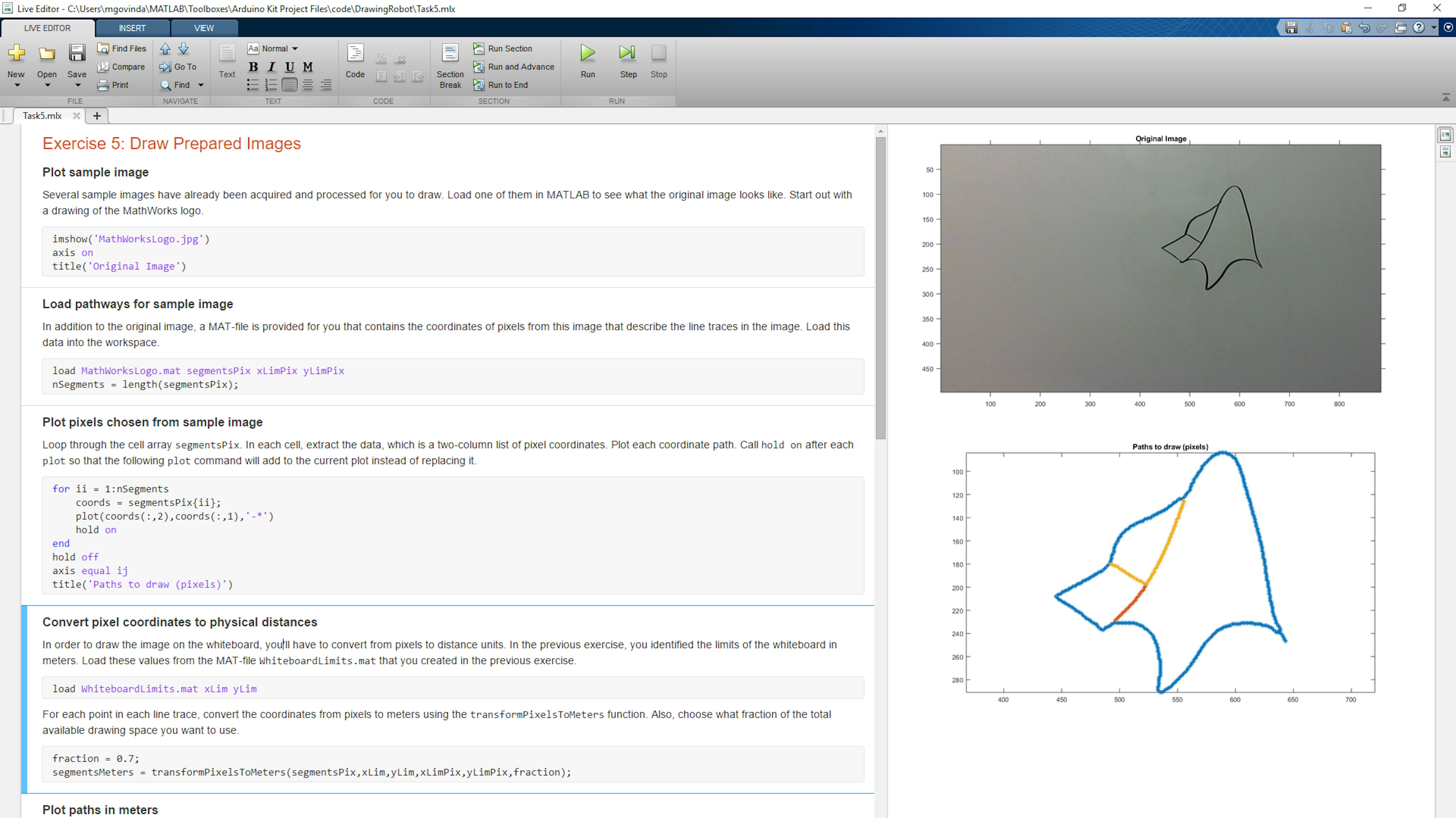
Next, you'll create a plot of the data in the segmentsMeters variable just as you plotted the data in the segmentsPix variable earlier. The resulting plot should look the same but use units of meters and a range within the limits of your whiteboard. Run the code in the Plot paths in meters section of Task5.ml.
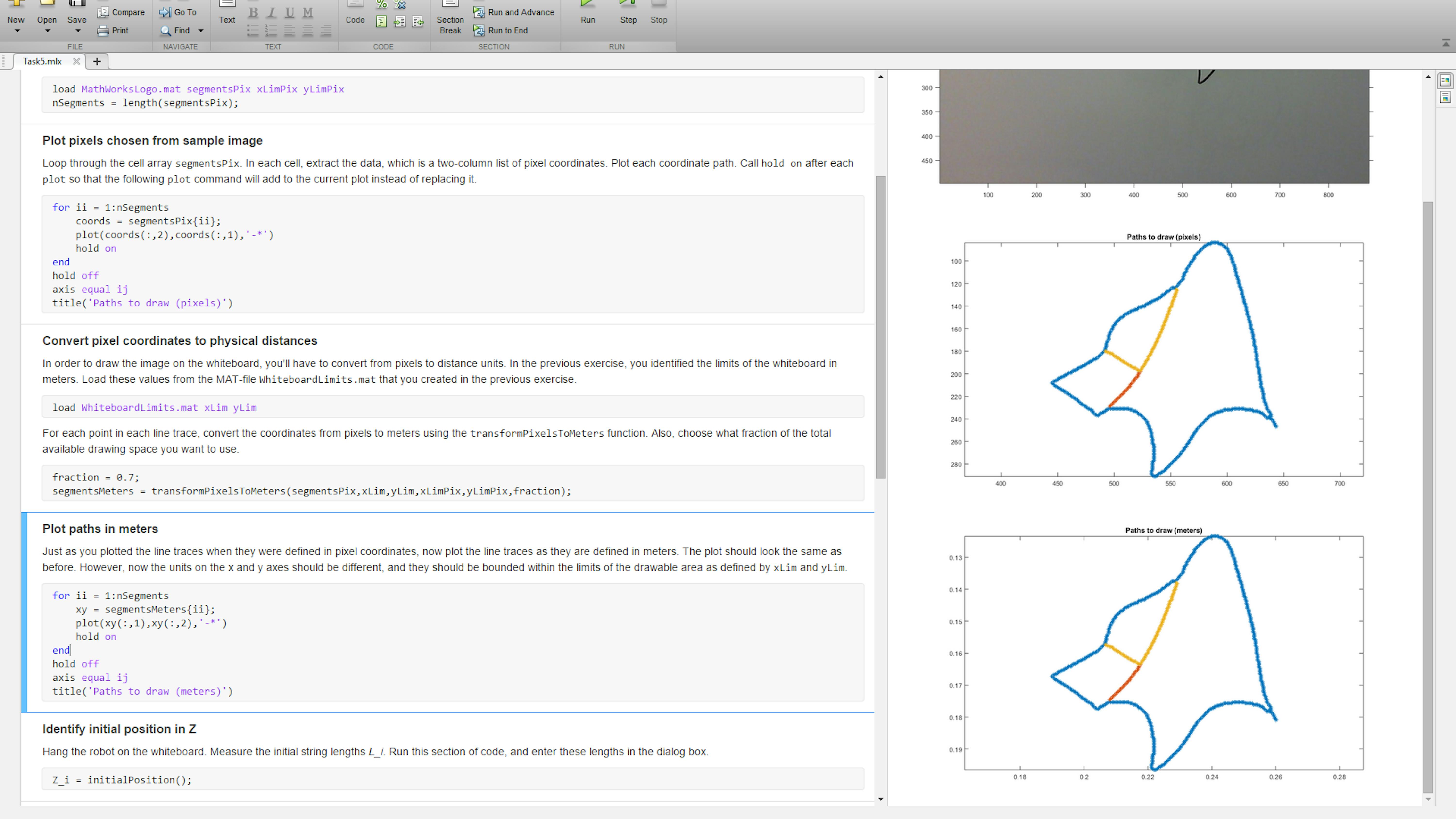
If you zoom in on this plot and use the Data Cursor, you’ll see that the points to be drawn are very close to each other (in this case most points are separated by less than 1 mm).

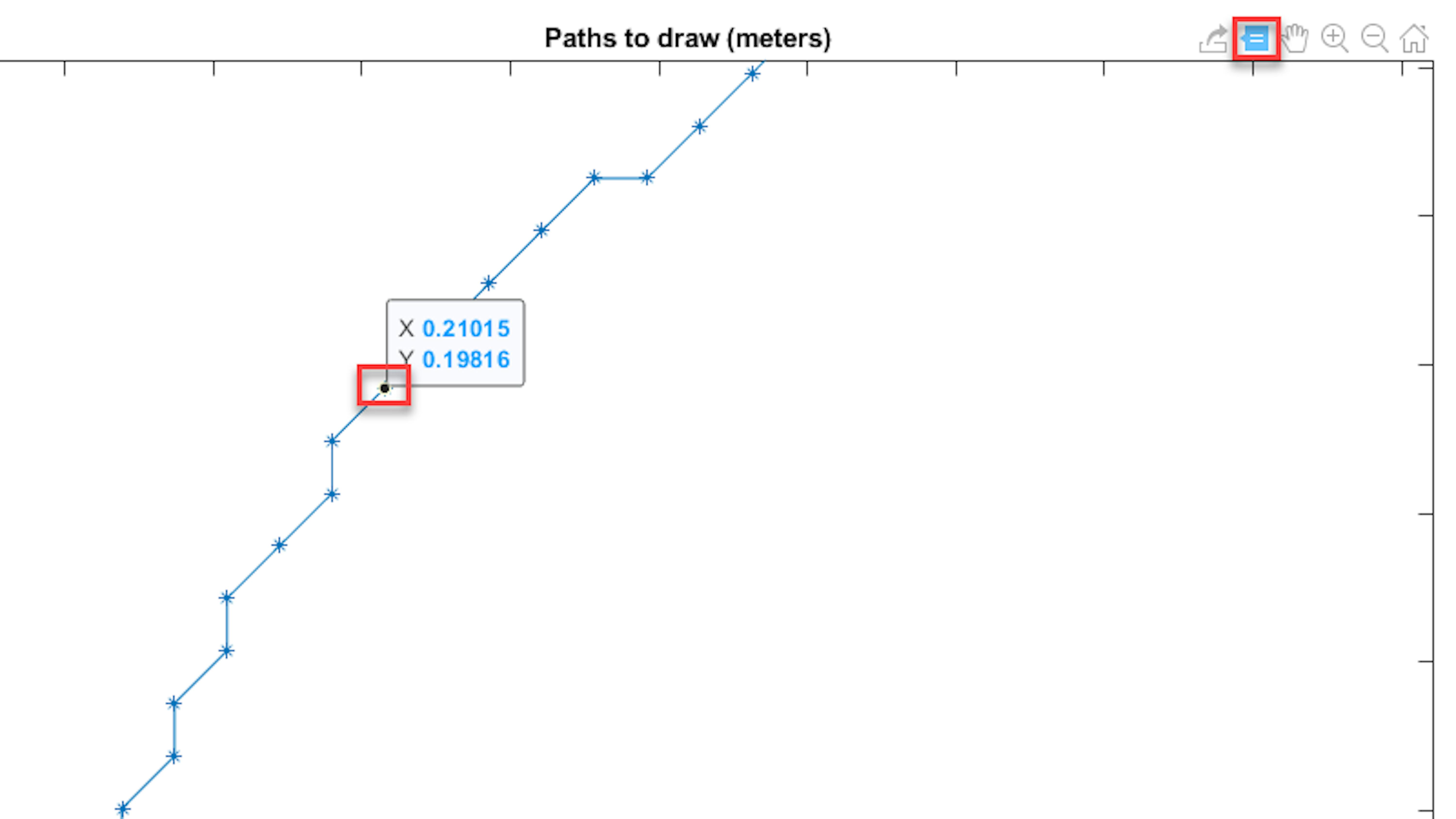
If the robot tries to draw each point on each segment, it will take a lot of time to finish the drawing. In the next section, we will see how to filter the segments to reduce the drawing time, while maintaining the fundamental shape of the image.
UNDERSTAND THE REDUCESEGMENT FUNCTION, LINE BY LINE
The reduceSegment function reduces the number of points in a segment by removing points within a specified radius. In other words, it filters out points, what reduces the amount of subsegments to draw. The function accepts two inputs: the segment that should be reduced and a radius value. The radius value is the desired minimum distance between any two points on the segment. As you read through, note how the function applies some of the concepts you learned previously, such as: while loop and logical indexing.
This function computes the scale factor for converting pixels to meters, then converts all the segments
in segmentsPix to meters.


function segmentsMeters = transformPixelsToMeters(segmentsPix,xLim,yLim,xLimPix,yLimPix,fraction)
First, create variables to represent the ranges xRange, yRange, xRangePix, and yRangePix.
xMinM = xLim(1);
yMinM = yLim(1);
xRangeM = diff(xLim);
yRangeM = diff(yLim);
% Determine the range of the coordinates to draw
xMinPix = xLimPix(1);
yMinPix = yLimPix(1);
xRangePix = diff(xLimPix);
yRangePix = diff(yLimPix);Calculate the two possible scale factors. The fraction factor indicates what percentage of the available
space should be used.
% Scale from pixels to real world units (meters)
xScaleFactor = fraction*xRangeM/xRangePix;
yScaleFactor = fraction*yRangeM/xRangePix;Choose the smaller of the two scale factors.
% Pick the smaller scale factor. If both are NaN, pick
0.
pix2M = min(xScaleFactor,yScaleFactor);
if isnan(pix2M)
pix2M = 0;
endBased on the chosen scaling factor and range values, identify the new origin for the scaled drawing
so that the full drawing will be centered at the center of the drawable area.
% Identify origin position of scaled drawing
centerMeters = [xMinM yMinM] + [xRangeM yRangeM]/2;
drawingOriginM = centerMeters - pix2M*[xRangePix yRangePix]/2;Loop through all segments and transform pixel values to meters for all coordinates. Subtract the pixel origin,
multiply by the scaling factor, and add the drawing origin.
segmentsMeters = cell(size(segmentsPix));
nSegments = length(segmentsPix);
for ii = 1:nSegments
% Scale all segments by the computed scaling factor
coordsPix = segmentsPix{ii};
coordsPix = fliplr(coordsPix); %Convert from row,col to x,y
coordsMeters = pix2M*(coordsPix-[xMinPix yMinPix]) + drawingOriginM;
segmentsMeters{ii} = coordsMeters;
endREDUCE SEGMENT SIZES AND PLOT
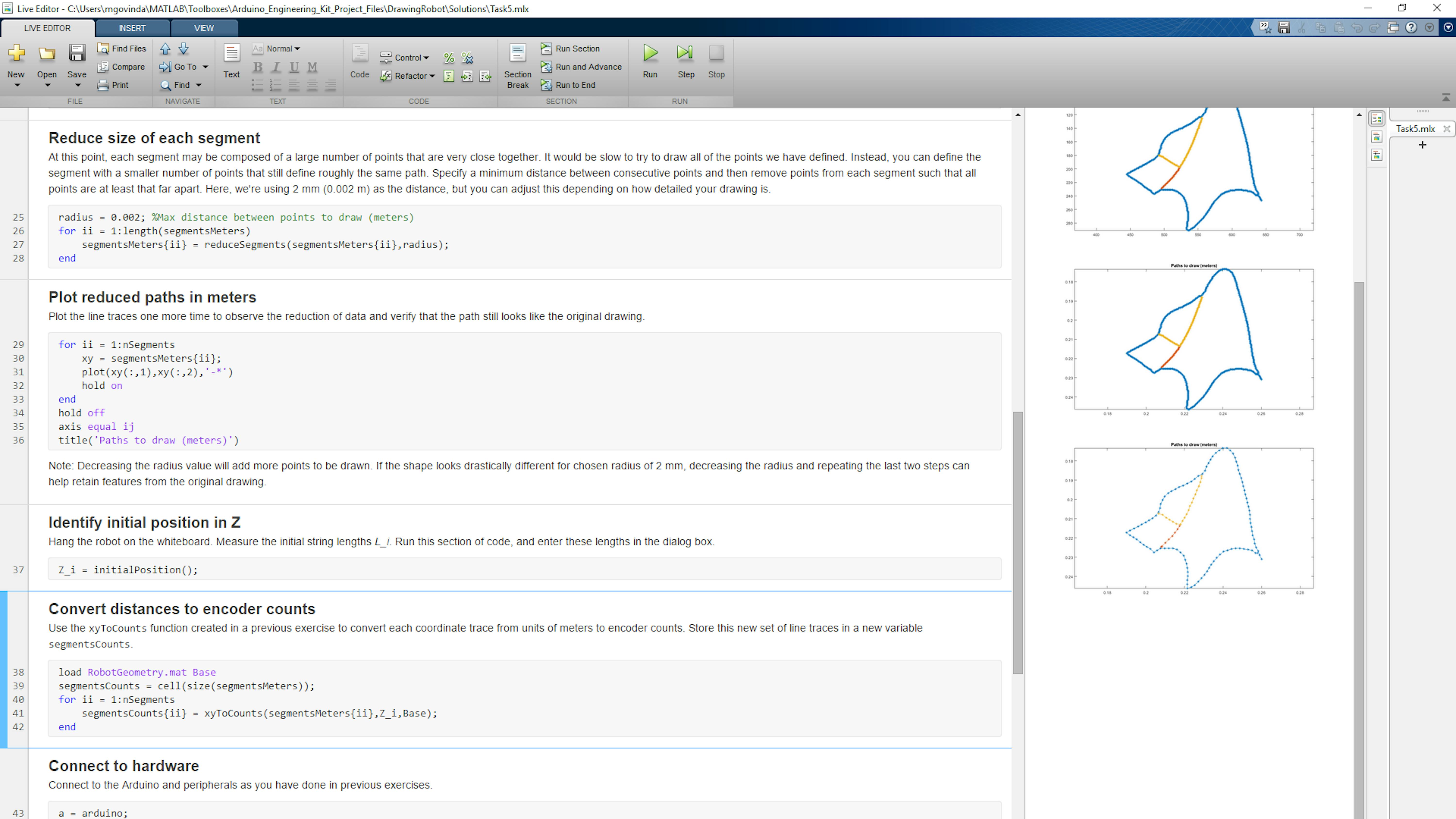
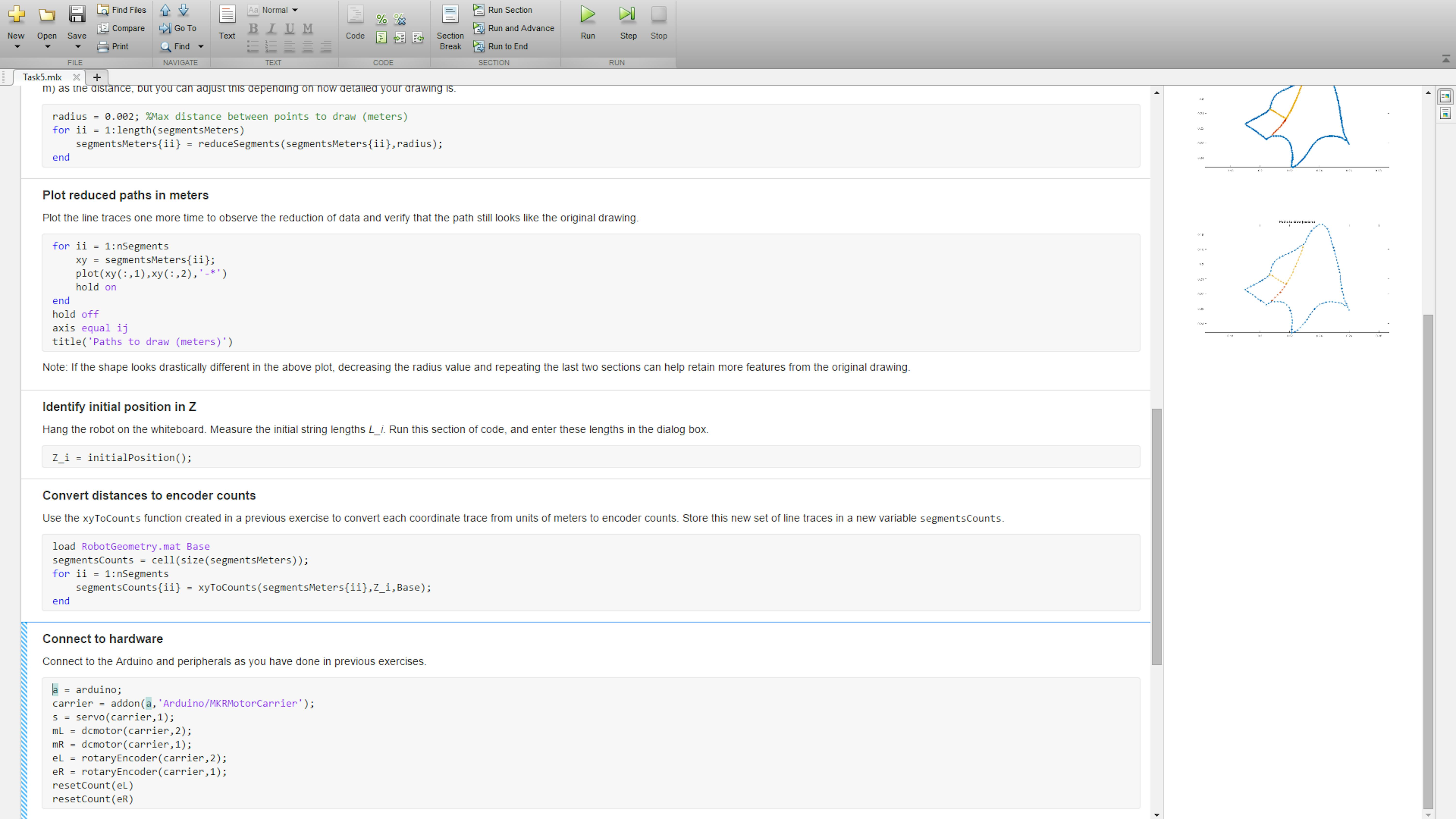
Let’s execute the reduceSegment function in a for loop to reduce the number of points in each segment of this image. Run the section of code under the heading Reduce size of each segment. Then run the section of code under the heading Plot reduced path in meters to visualize the updated paths.
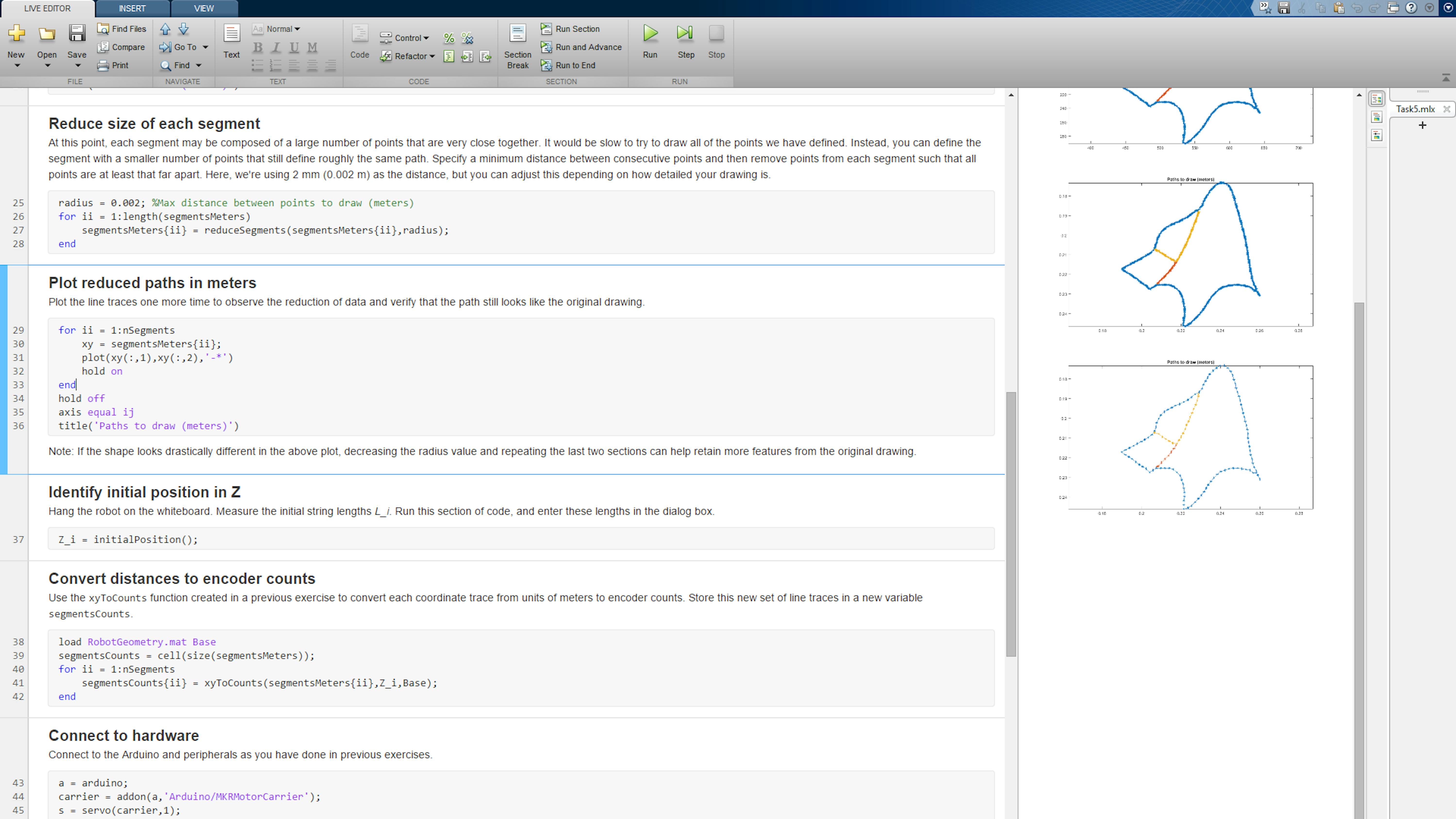
This will represent a third plot, where you will see a lot less points, what will significantly reduce the time to print such an image with the robot.
Note: The empirically-obtained radius value of 2 mm worked well for images on our whiteboard. If the image on your whiteboard looks like it is missing important features, try decreasing the radius and running the last two sections of code again. Alternatively, if your image doesn’t have much fine detail, you may be able to draw it even faster by choosing a larger radius. Choosing a radius value that balances drawing speed and reproduction accuracy is at this point a process of trial and error. You could consider improving this algorithm in several ways: by figuring out how different an image is from one another, and by having a dynamic radius depending on the estimated error between the original and reduced images.
CONVERT DESIRED POSITIONS TO ENCODER COUNTS
As you did in a previous exercise, you'll now use the xyToCounts function to convert the target positions in meters to encoder counts. Before running this function, you'll have to determine the initial position of the robot. Measure the length of each string as you've done in previous exercises. Then run the section of code under the heading Identify initial position in Z and enter these lengths in the dialog box.
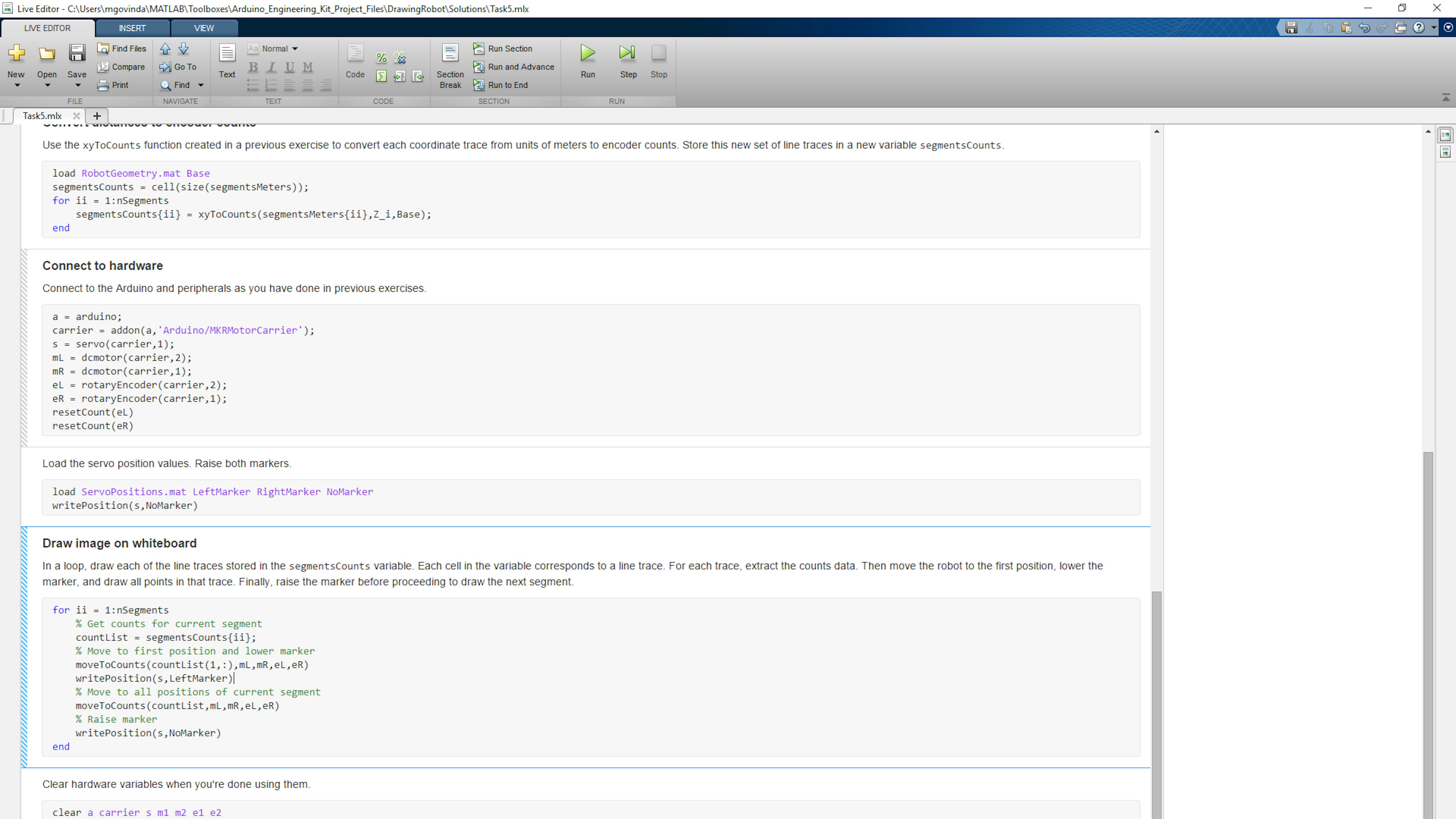
Because the data is stored in a cell array, you'll have to loop through the array with a for loop and convert the pathways one at a time. Store the resulting encoder count targets in a cell array called segmentsCounts. Run the code under the heading Convert distances to encoder counts in Task5.mlx.
DRAW LINE SEGMENTS ON WHITEBOARD
Now that you have the encoder counts for all the positions you want to move the robot to, you can use these to draw each path just as you did in a previous exercise. As before, first connect to the hardware. Run the code sections under the heading Connect to hardware in Task5.mlx.
Look at the code in the section Draw image on whiteboard. It uses a for loop to step through the segmentsCounts variable. Think about what's happening in the loop. Each iteration of the loop applies to one of the line traces in the image. It extracts the encoder counts for that line trace, moves the robot to the first position, lowers the marker, then moves the robot to all positions in that line trace, and finally raises the marker. This is repeated for each of the three traces in the image. Run this section of code to draw the image on the whiteboard.
WRITE A FUNCTION FOR DRAWING AN IMAGE FROM PIXELS
You've completed a task that started with data about the pixels in an image to plot and ended with drawing the image on a whiteboard. If you want to perform all these steps again, it's useful to have this code bundled together in a function. Create a new MATLAB function and call it drawImageFromPix.m . The function will take pixel data and whiteboard starting position as inputs and then draw the image. Include the following code in the function and save it.
function drawImageFromPix(segmentsPix,xLimPix,yLimPix,Z_i)
nSegments = length(segmentsPix)

% Define whiteboard limits
load WhiteboardLimits.mat xLim yLim

% Convert pixel coordinates to physical distances and then to encoder counts
fraction = 0.7;
segmentsMeters = transformPixelsToMeters(segmentsPix,xLim,yLim,xLimPix,yLimPix,fraction);

% Reduce size of each segment
radius = 0.002; %Max distance between points to draw (meters)
for ii = 1:nSegments
		segmentsMeters{ii} = reduceSegment(segmentsMeters{ii},radius);
end

load RobotGeometry.mat Base
segmentsCounts = cell(size(segmentsMeters));
for ii = 1:nSegments
segmentsCounts{ii} = xyToCounts(segmentsMeters{ii},Z_i,Base);
end

% Connect to hardware
a = arduino;
carrier = addon(a, 'Arduino/MKRMotorCarrier' );
s = servo(carrier,3);
m1 = dcmotor(carrier,2);
m2 = dcmotor(carrier,1);
e1 = rotaryEncoder(carrier,2);
e2 = rotaryEncoder(carrier,1);
resetCount(e1)
resetCount(e2)

% Define up and down positions for servo motor
load ServoPositions.mat LeftMarker NoMarker

% Draw image on whiteboard
writePosition(s,NoMarker)
for ii = 1:nSegments
% Get counts for current segment
countList = segmentsCounts{ii};

% Move to first position and lower marker
moveToCounts(countList(1,:),m1,m2,e1,e2)

writePosition(s,LeftMarker)

% Move to all positions of current segment
moveToCounts(countList,m1,m2,e1,e2)

% Raise marker
writePosition(s,NoMarker)
end
The variables segmentsPix , xLimPix , yLimPix , and Z_i should still be in your Workspace. Run your new function at the MATLAB command prompt to draw the image again and confirm that the function works as expected.
>> drawImageFromPix(segmentsPix,xLimPix,yLimPix,Z_i)
FILES
- Task5.mlx
- transformPixelsToMeters.m
- drawImageFromPix.m
LEARN BY DOING
In this exercise, you drew an image using data from the MathWorksLogo.mat MAT-file. Other MAT-files have been provided for you, containing the line traces from other images. Update your code to draw some of these other images. Preview how they will look in MATLAB, and then draw them on the whiteboard.
For a more advanced challenge, try drawing two images side by side. Load the MAT-file data for both images. Then update the data from the second image so that its pixel coordinates are to the right of all points in the first image. Then concatenate the cell arrays of pixel positions. Finally, update the xLimPix and yLimPix variables so they accurately describe the pixel limits for the new combined set of paths.
EXERCISE 6:
4.6 Draw any image
In the previous exercise, you took a set of pixel positions that described pathways in an image and used the drawing robot to draw those pathways. Now you'll learn how to take a photograph and process the image to identify those pixel positions and pathways to draw. You'll use image conversion, filtering, and analysis techniques. When you're done, you'll be able to use your robot to recreate any image with a line drawing. Try drawing the included sample images or make your own.
In this exercise, you will learn to:
- Convert, filter, and analyze images using image processing functions
- Construct recursive functions
- Simplify code by operating on entire array at once
- Write a main script to run whole workflow
UNDERSTAND IMAGE CONVERSION, FILTERING, AND ANALYSIS
Image Processing Toolbox provides a large amount of functionality for image processing, analysis, visualization, and algorithm development. For this project, you'll leverage some of these capabilities to take an image of a line drawing and extract the line traces.
In a previous exercise, you saw that an image can be represented in MATLAB as an MxNx3 array of uint8 values, which is great if you want to preserve all the information about an image. This is just one of several ways to represent an image. We can reduce the complexity of an image to extract the specific information we are interested in. Here are some other forms an image can take in MATLAB.
- A color image can also be represented as a 2-dimensional MxN array with a corresponding colormap. We won't be working with this type of color image.
- A grayscale image can be represented simply as an MxN array. This is useful for image processing functions that operate on a 2-D grid of data, such as filtering.
- A binary image can be represented as an MxN array of logical (true or false) values. This is useful for extracting characteristics of particular regions in an image.
If you want more information about image processing, you can check this book.
Let's examine an image and convert it to grayscale. Run the following code at the MATLAB command prompt to load and view the peppers image in MATLAB:
>> RGB = imread('peppers.png');
>> imshow(RGB);
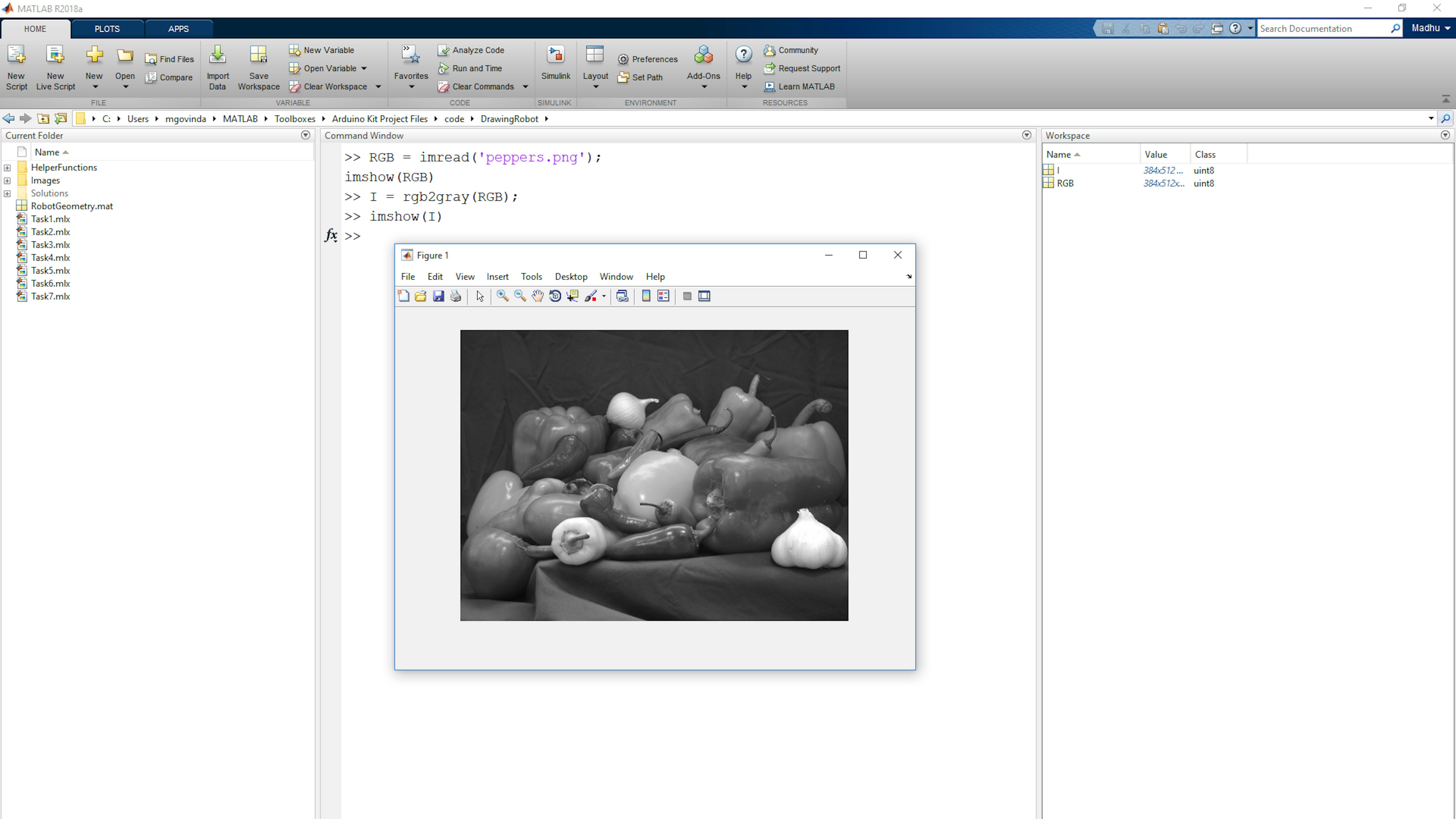
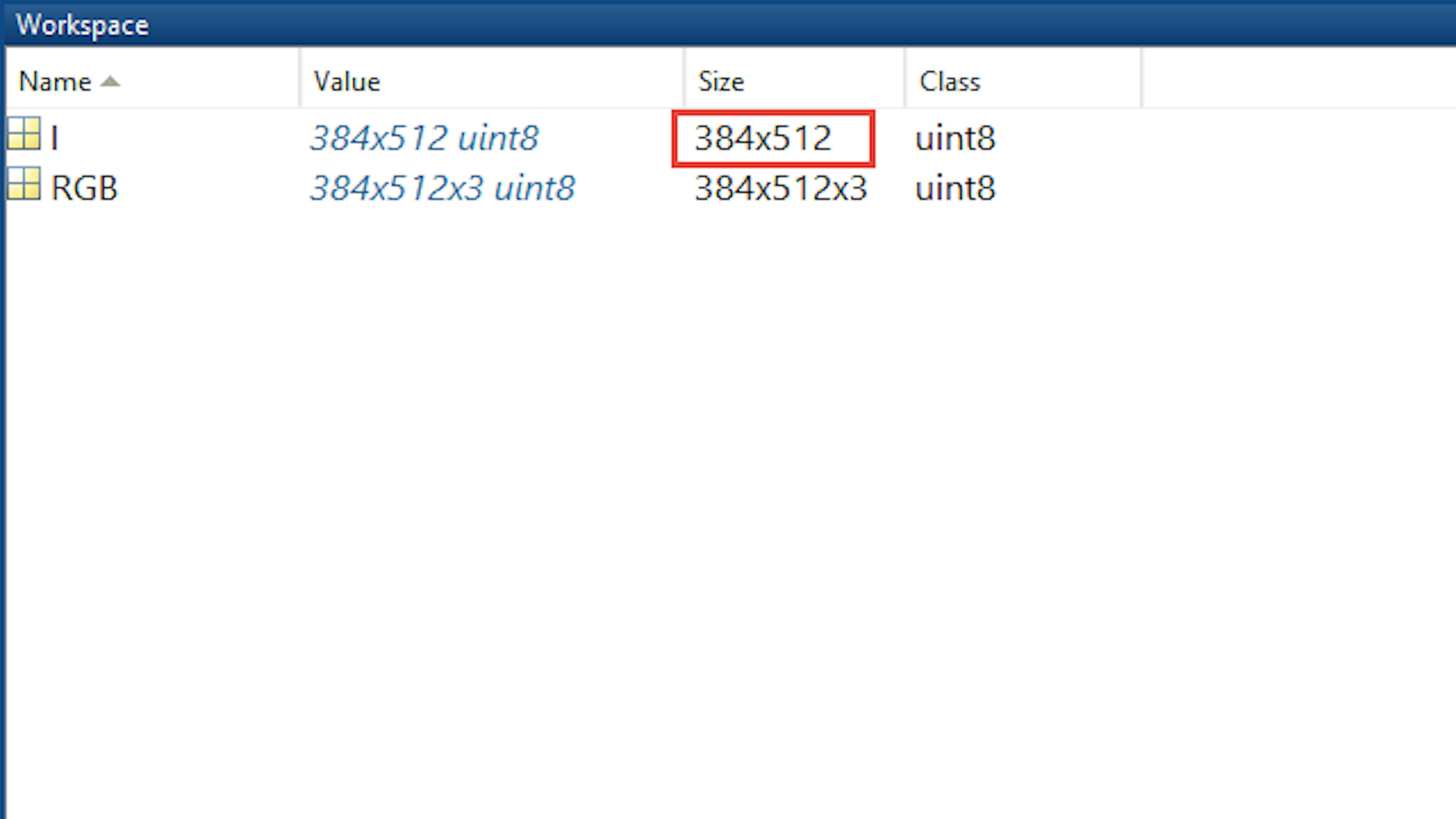
Now convert the image to grayscale and view it. Also, note the dimensions of the new image in the MATLAB workspace.
>> I = rgb2gray(RGB);
>> imshow(I)
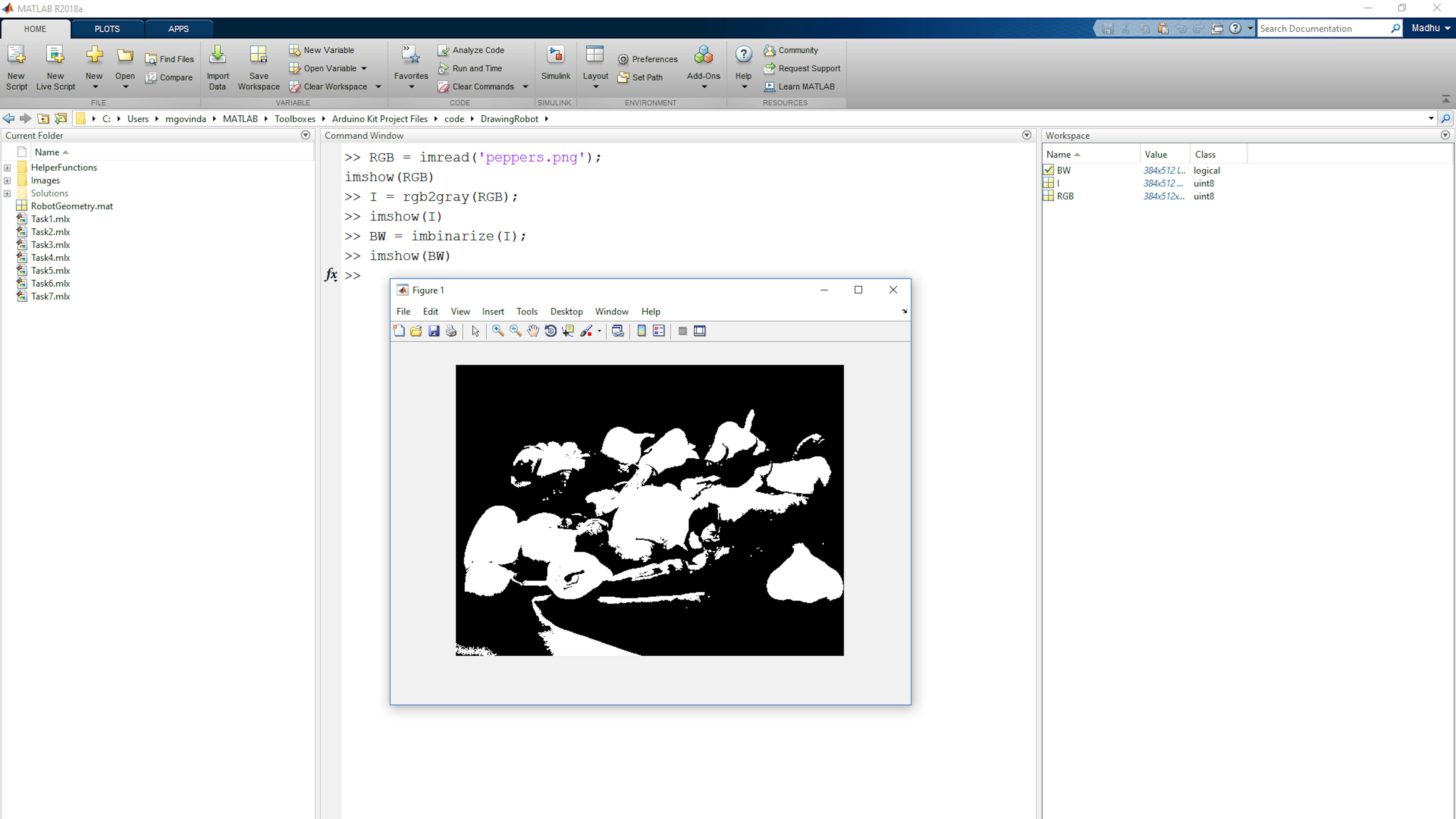
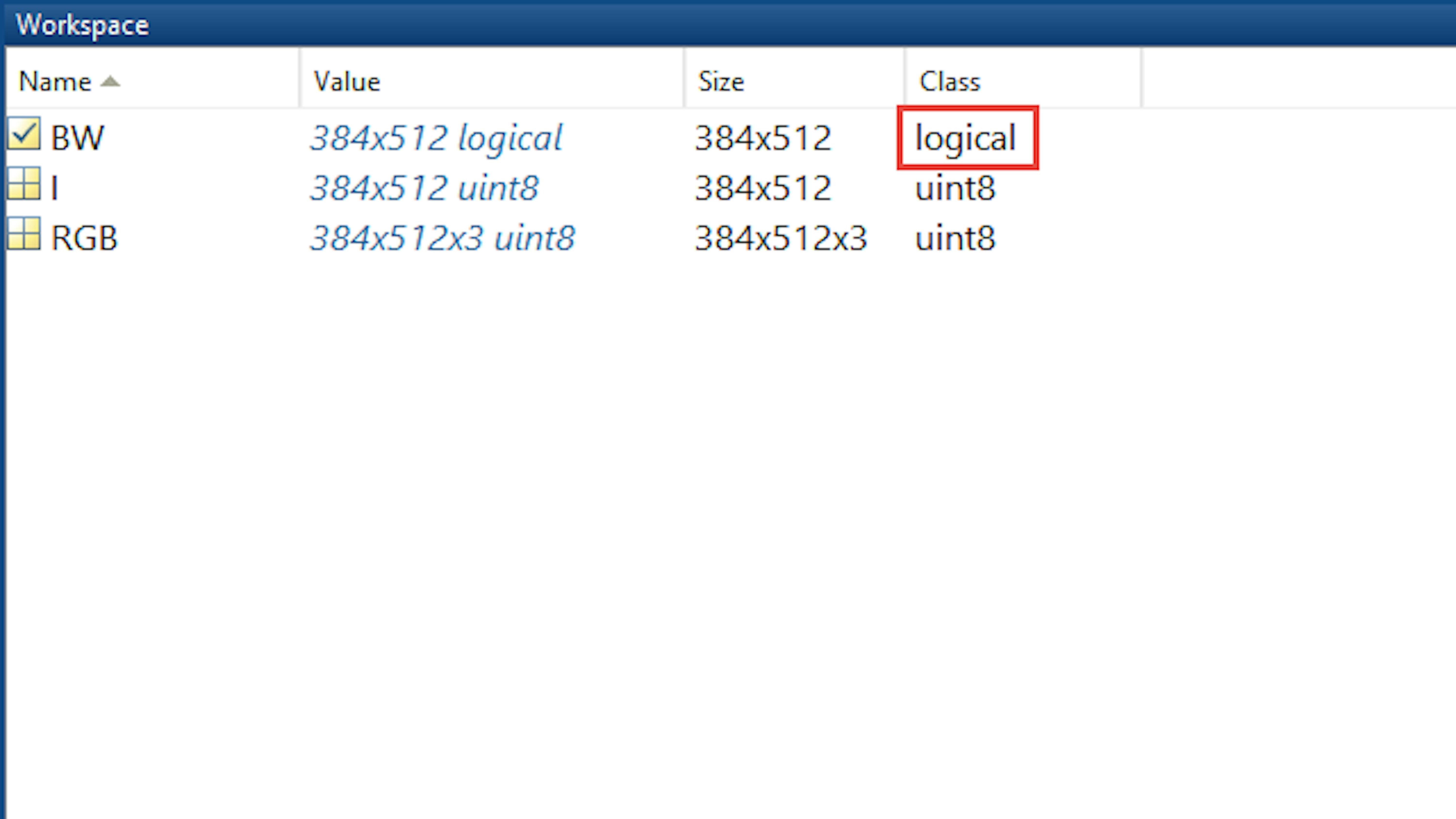
Binary images are images where each pixel is either on or off. These are visualized in pure black-and-white, which can be useful for describing specific regions or objects in an image. A grayscale image can be converted to binary using the imbinarize function. This function replaces all values above a certain threshold with 1 and those below that threshold with 0. The threshold can be global or regional. Convert the peppers image to binary and view it. Also, note the data type of the binary image.
>> BW = imbinarize(I);
>> imshow(BW)
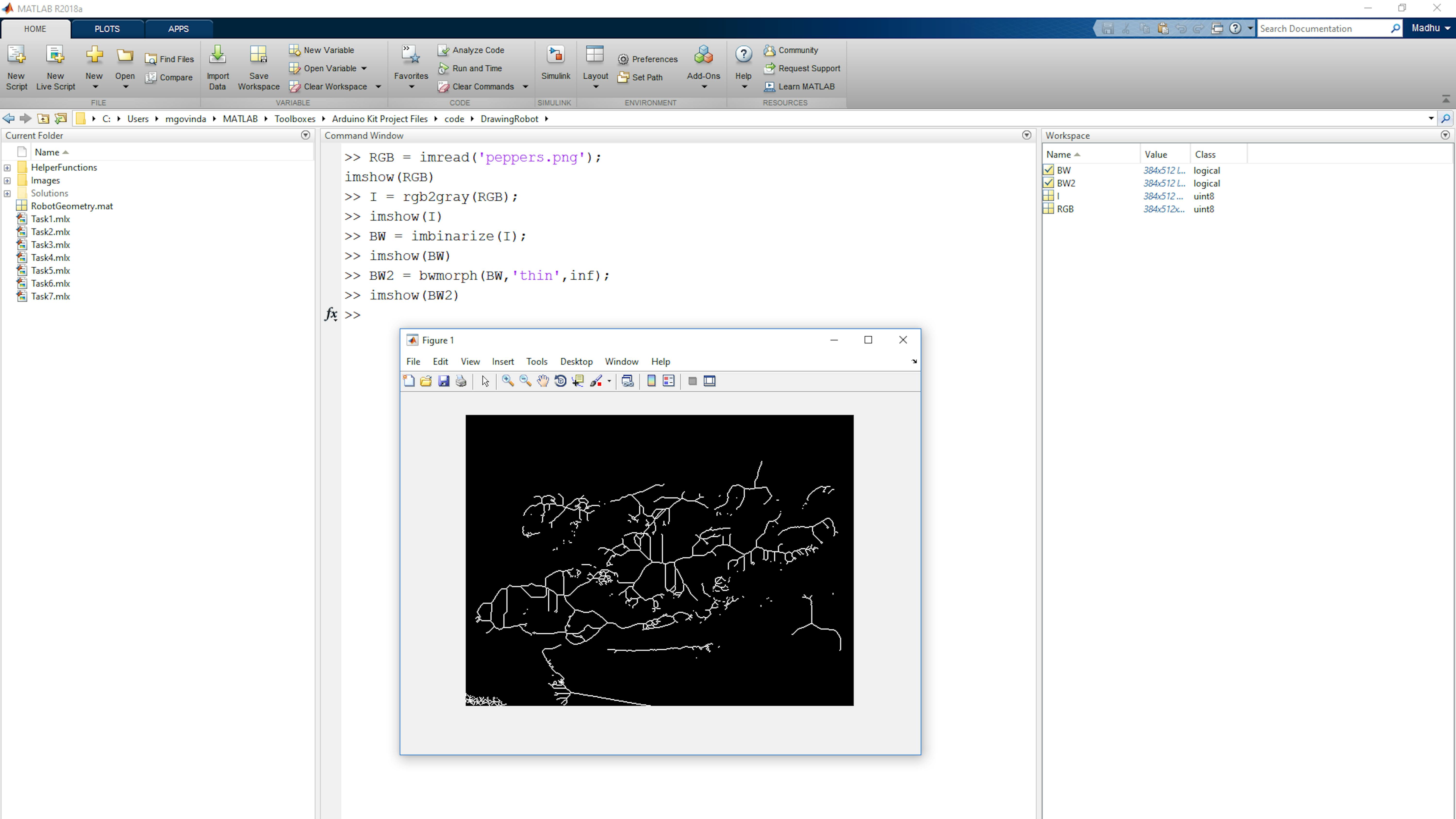
There are many ways you can process binary images to extract the features you want. One approach is to use morphological operations such as dilation and erosion. The most useful of these for extracting line traces is the thinning operation. This can thin objects in the image all the way down to lines. Test this out on the peppers image to see what line traces represent the thinnest version of the objects shown in this image.
>> BW2 = bwmorph(BW,'thin',inf);
>> imshow(BW2)
See the following MATLAB documentation pages for more information about these and other image processing functions:
In the following sections, we'll use the same techniques to extract line traces from raster images.
LOAD EXISTING IMAGE FROM FILE
You can use functionality from Image Processing Toolbox to convert any image into a form that is drawable by a robot. First, try this on the provided sample images. Later, you can try using your own photos.
Start by loading an image into MATLAB. We'll use a line drawing of the MathWorks logo. Open Task6.mlx in MATLAB.
>> edit Task6
Run the first section of the live script under the heading Load image from file.
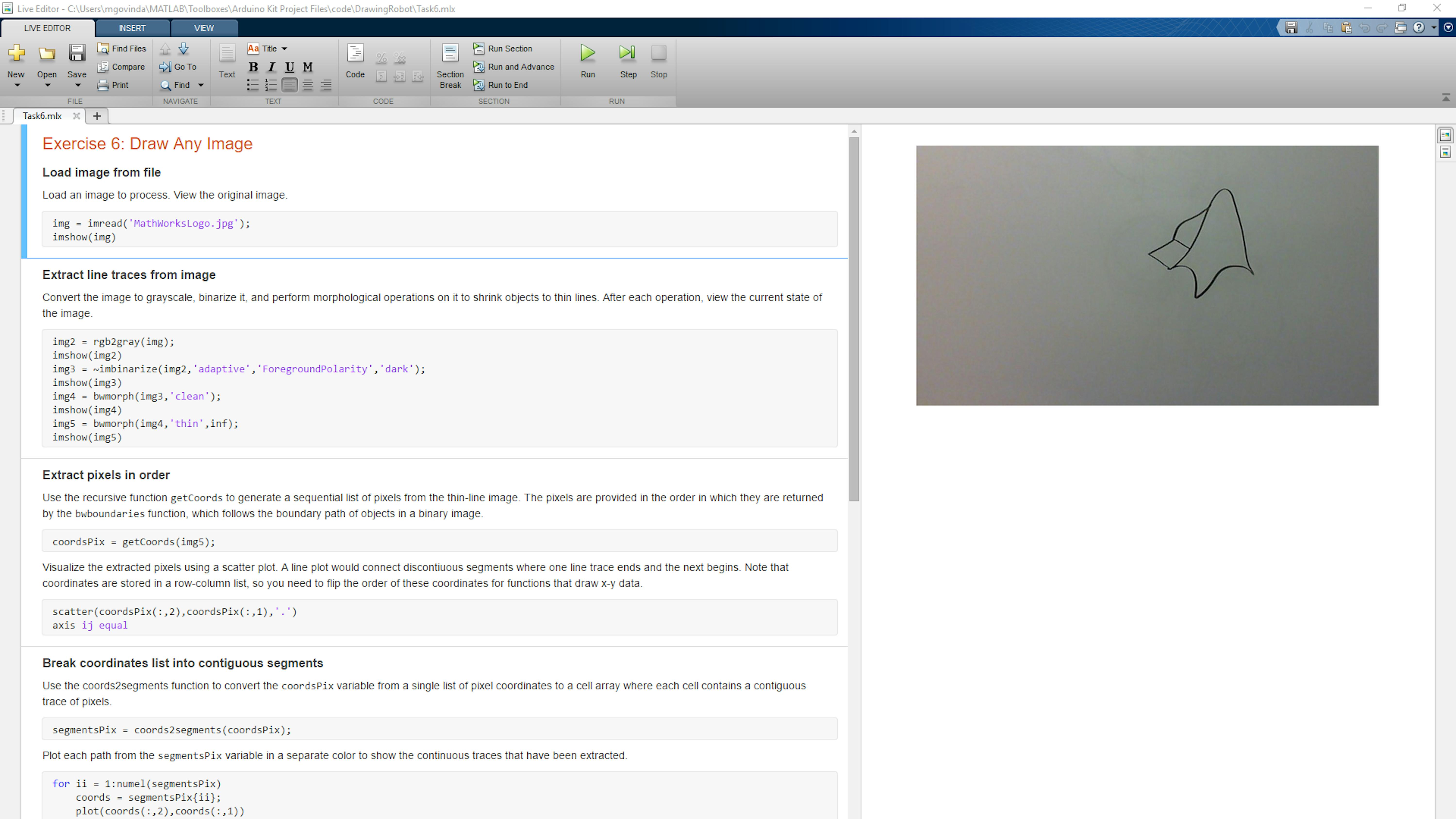
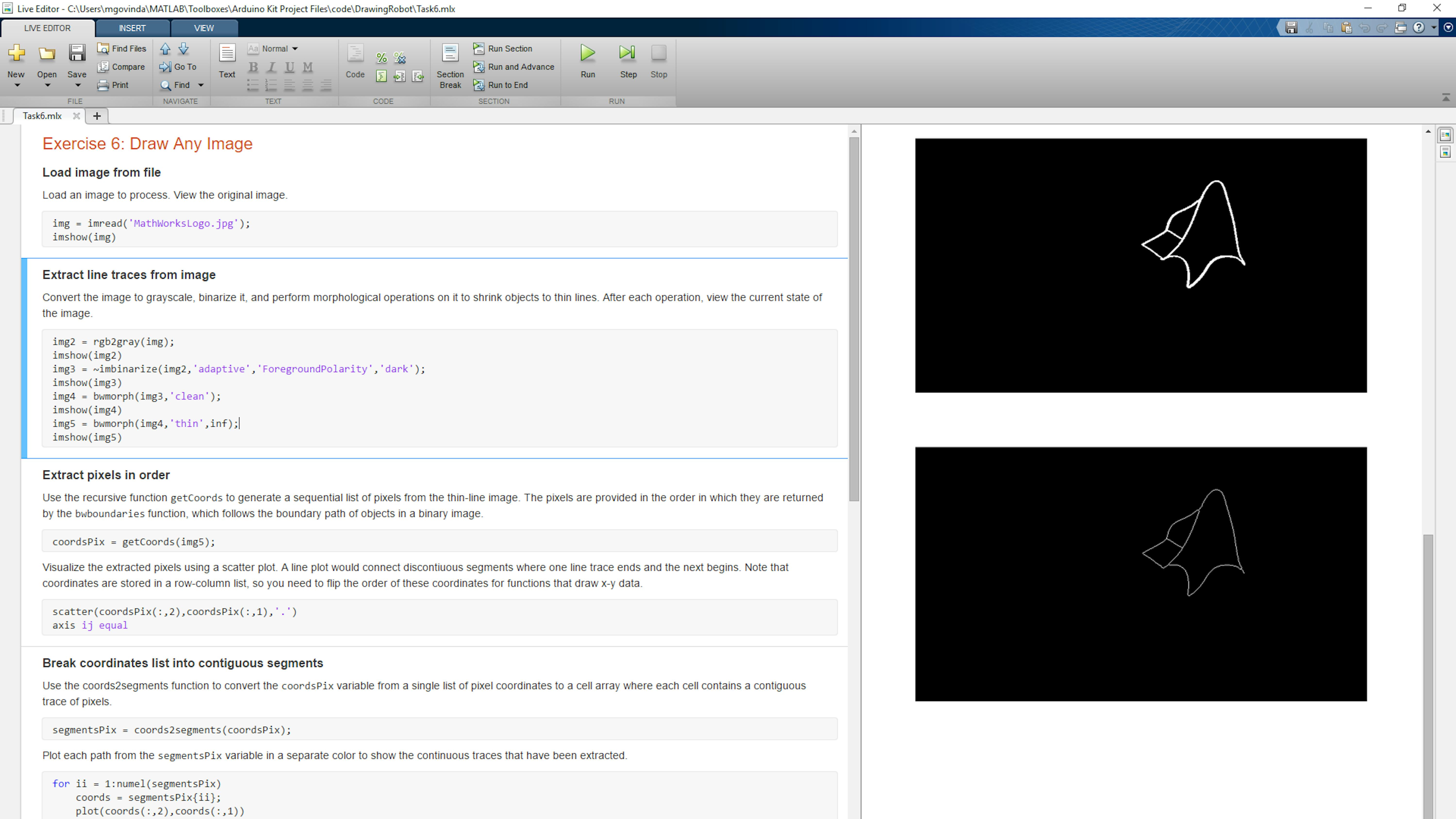
EXTRACT LINE TRACES FROM IMAGE
Process the image so that it contains only the thin traces of lines. Use image processing functions to convert the image to grayscale, convert it to binary black and white, remove isolated pixels, and thin objects to lines. Do this by running the section of Task6.mlx under the heading Extract line traces from image. The output of the live script shows what the image looks like after each step.
UNDERSTAND RECURSIVE FUNCTIONS
So far, you should be familiar with MATLAB functions that take inputs and return outputs. Sometimes another instance of that function can be called from within a function. This is called a recursive function. Recursive functions can be useful when you want to solve a problem by iteratively breaking it down into a simpler version of itself. When you get to the simplest or base case, you return the simplest value. To illustrate how this works in practice, consider how you compute a factorial. This is defined by a product series:
$n!=\prod_{i=1}^ni=1{\cdot}2{\cdot}3{\cdot}{\dots}{\cdot}n-1{\cdot}n$
Note that this definition contains within it the definition of ( n - 1)!
$n!=1{\cdot}2{\cdot}3{\cdot}{\dots}{\cdot}n-1{\cdot}n=\left(n-1\right)!{\cdot}n$
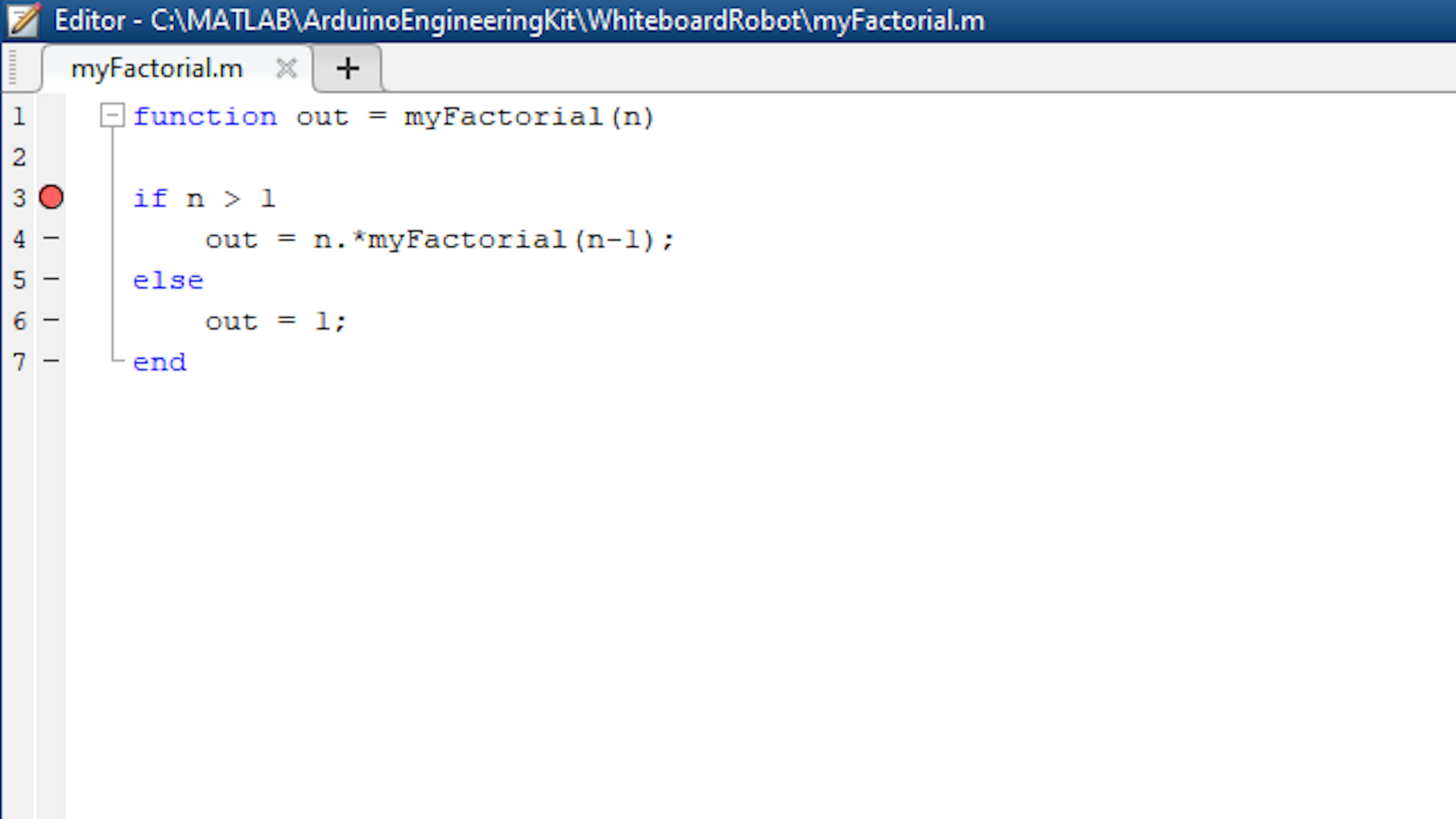
Therefore, one possible way to compute n! is to iteratively compute ( n - 1)! until you reach the simple case where n = 1. In MATLAB, a recursive function to do this could be written as follows:
function out = myFactorial(n)

if n > 1
	out = n\*myFactorial(n-1);
else
	out = 1;

end
This function multiplies n with the factorial of n - 1. But when MATLAB must compute the factorial of n - 1, it creates a new instance of the myFactorial function to do so. This repeats until the function is computing the factorial value for 1. Then, instead of creating a new recursive instance, it simply returns 1 and then steps back up the stack until the result is computed and returned for the first call to myFactorial . To see how this works, create the above function in MATLAB and add a breakpoint to the first line by clicking the dash (-) next to the line number.
Now call the function from the MATLAB command prompt:
>> myFactorial(4)
The debugging breakpoint will be hit. Click the Step button on the Editor toolstrip to move through the code and keep hitting the breakpoint on subsequent instances of myFactorial that are called. After each step, check the Workspace to see the current values of n and out . You can also check the Function Call Stack to see which instance of myFactorial is currently running.
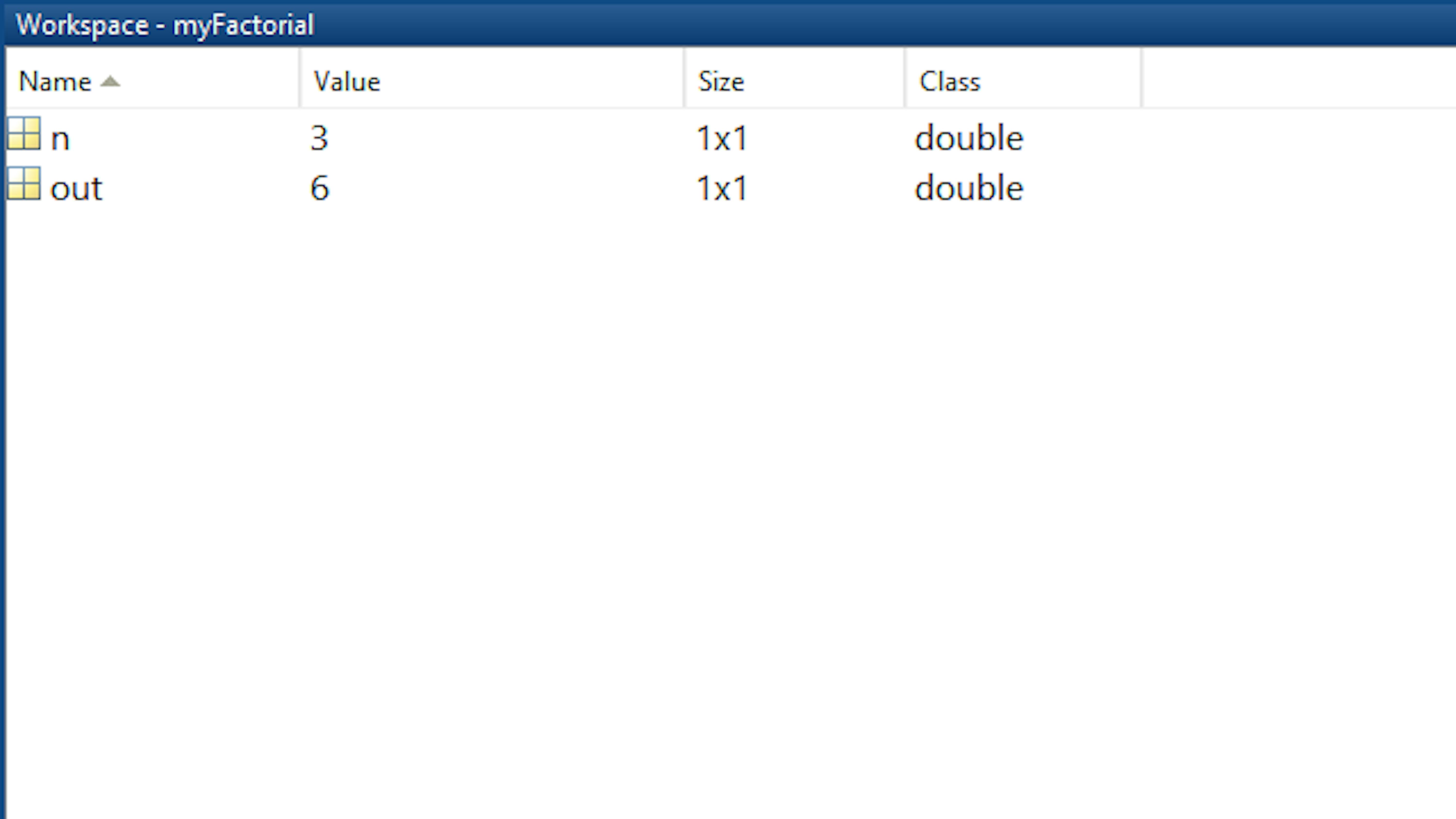
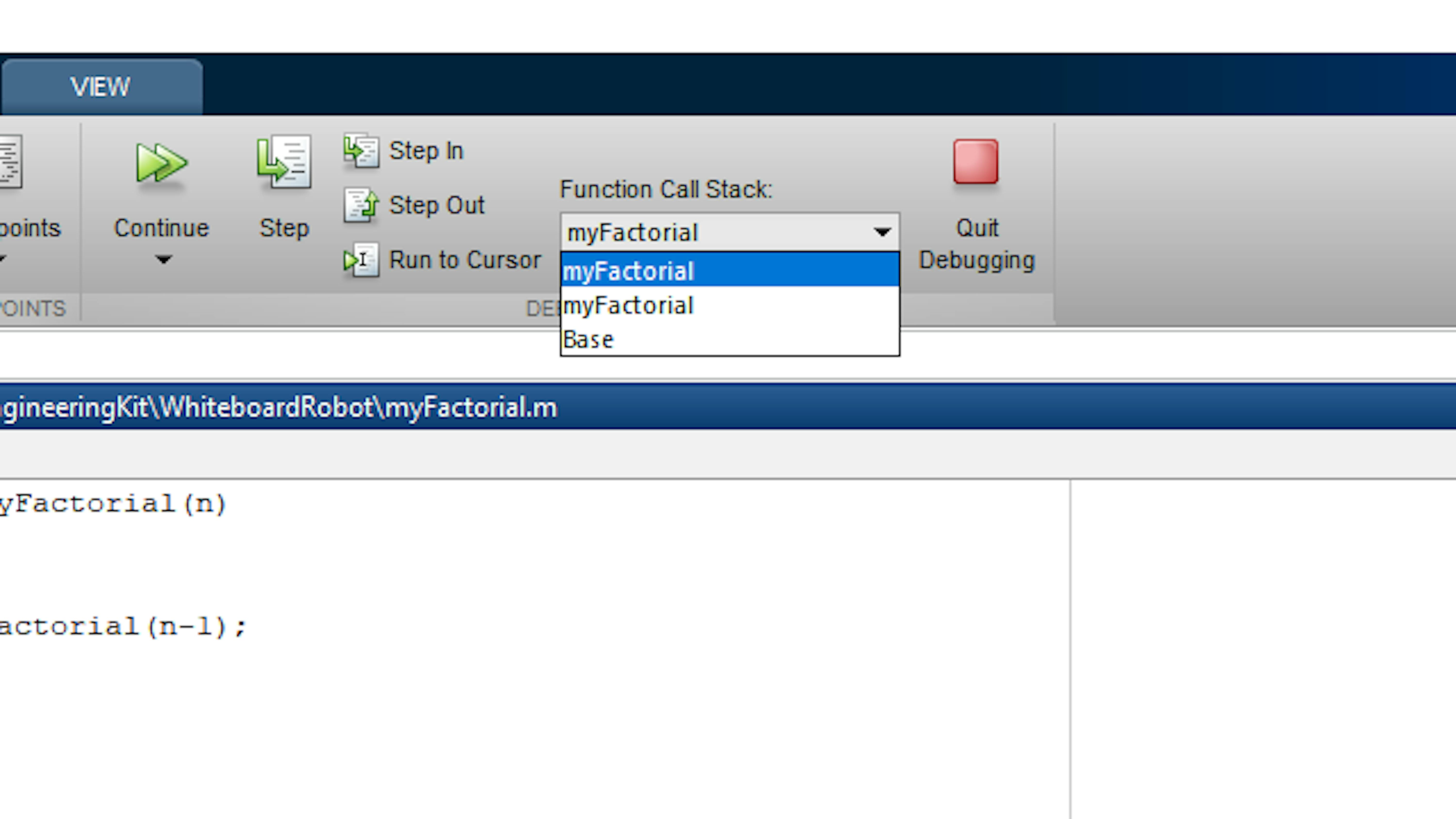
This is just an illustration of recursion and is not the most efficient way to compute a factorial. In MATLAB, an easy way to do this is to simply use the prod function on the full sequence 1 to n.
>> prod(1:4)
UNDERSTAND THE GETCOORDS FUNCTION, LINE BY LINE
To extract the traces from an image in the form of pairs of coordinate values that compose curves, we have created the getCoords function. It is a recursive function that continues to call itself while there are still pixels available on a binarized image and concatenates them into a single array.
This function calls bwboundaries recursively, stripping off the outer pixel boundaries
from the image each time and concatenating them.


function curvePoints = getCoords(shapeImage)
First, call bwboundaries to get the boundaries of each unique region.
% Detect boundary points
[curves,~,N] = bwboundaries(shapeImage);
curves = curves(1:N); % Ignore hole boundariesGet the pixels from the boundaries.
% Get the points from the boundary detected
curvePoints = cell2mat(curves);If there are any duplicate pixels, remove them, and keep only unique pixels.
% Remove all duplicate points from the curve
curvePoints = unique(curvePoints,'rows','stable');In the image you're analyzing, remove all the pixels that were captured by bwboundaries.
There may still be pixels remaining in the image.
% Remove curves from the image
curveInd = sub2ind(size(shapeImage),curvePoints(:,1), curvePoints(:,2));
shapeImage(curveInd) = 0;Check the image to see whether any pixels remain. If no pixels remain, return the curvePoints found.
If there are more pixels, call this function again and add curvePoints to the additional pixels found
by the recursive call.
% Call getCoords recursively if there are other curves remaining
if any(shapeImage(:))
curvePoints = [curvePoints; getCoords(shapeImage)];
endRECURSIVELY EXTRACT PIXELS IN ORDER
Now you can call getCoords on the image to extract the selected pixels from the image in an order that puts adjacent pixels next to one another. The output will be an Nx2 array of pixel coordinates that contains the result of each iteration of getCoords stacked on top of each other. N is the number of pixels identified in the image. You can also visualize these pixel coordinates on a scatter plot. Run the section of the live script Task6.mlx under the heading Extract pixels in order .
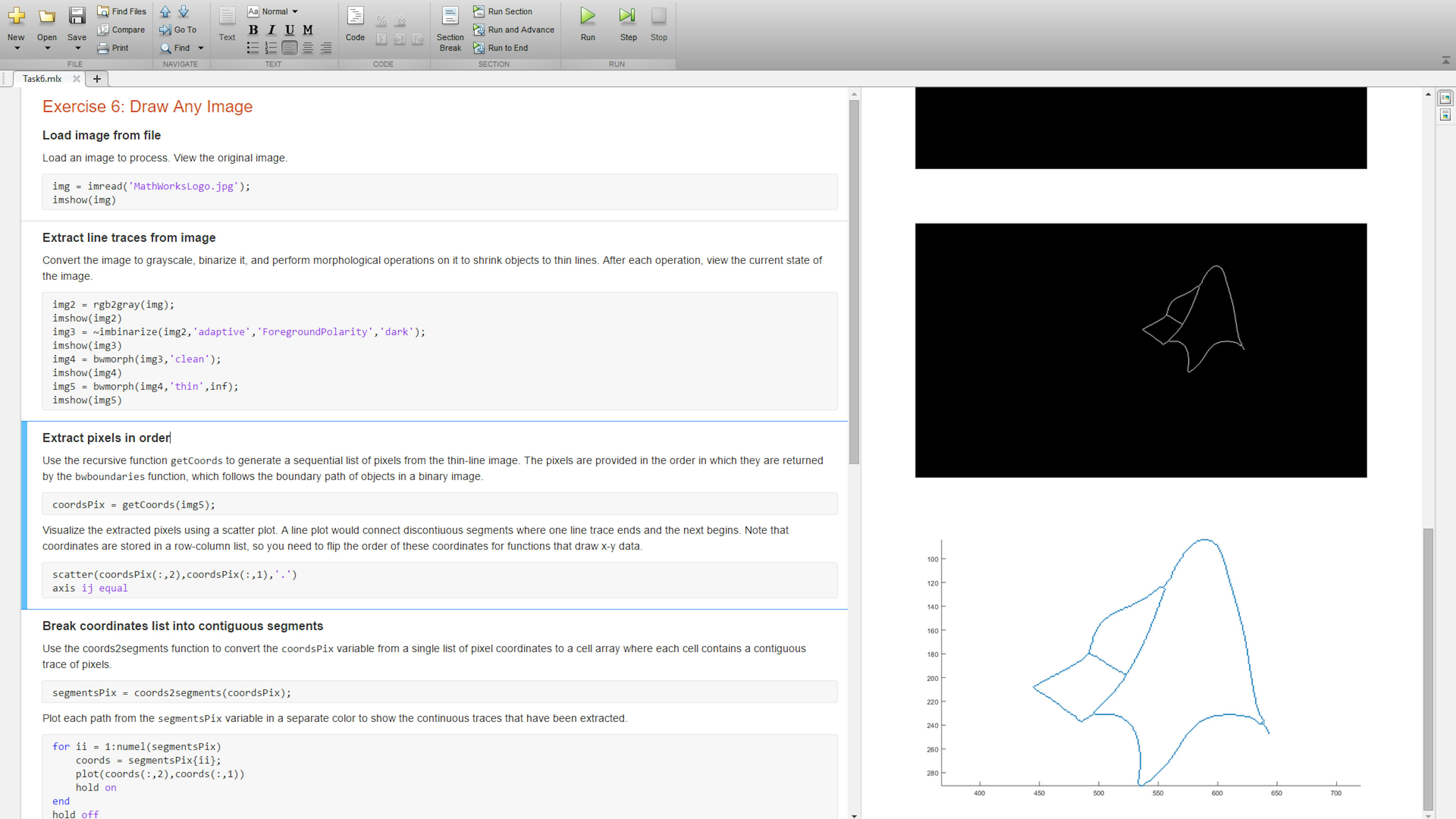
UNDERSTAND THE COORDS2SEGMENTS FUNCTION, LINE BY LINE
Given a sequence of data pairs obtained with the getCoords function, we need to identify the different sets of pixels. This is done by checking each pair of pixels to see if they are adjacent and then splitting them off if they are not. All the resulting segments are stored in a single cell array.
This function looks at every pair of pixels and determines where they are not adjacent. It then splits
coordsPix into sets of contiguous pixels, storing each in a separate cell as part of the cell array segmentsPix.


function segmentsPix = coords2segments(coordsPix)
First, find the places where consecutive pixels are not adjacent. Create a breaks variable that
is a logical index with 1 where there is a break and 0 where pixels are adjacent.
% Find discontinuous locations in coordsPix
consecutiveDistance = abs(diff(coordsPix));
breaks = any(consecutiveDistance > [1 1],2);Use the breaks variable to construct the indices of the start and end of each segment. Then loop through the
segments and create cell array segmentsPix , where each cell contains all the pixel coordinates for that segment.
% Build cell array of each segment of adjacent pixel coordinates
numSegments = sum(breaks)+1;
segmentsPix = cell(numSegments,1);
breakInds = [0; find(breaks); size(coordsPix,1)];
for ii = 1:numSegments
segmentsPix{ii} = coordsPix(breakInds(ii)+1:breakInds(ii+1),:);
endBREAK COORDINATES LIST INTO CONTINUOUS SEGMENTS
Now you will call coords2segments on the array of pixel coordinates extracted in the previous step. This will return a cell array where each element is a list of contiguous pixels. Plot each group of pixels to see which ones are organized together. Run the section of the live script Task6.mlx under the heading Break coordinates list into contiguous segments.

Notice how the red and blue traces share a common endpoint at the leftmost end. In the next section, we'll see how to combine these into a single line trace.
UNDERSTAND THE CONNECTSEGMENTS FUNCTION, LINE BY LINE
Given the results from the previous function, there might be segments with adjacent endpoints that could be merged with one another. This could reduce the total number of segments in the image.
The connectSegments function does two things. First, it closes any segments that intersect themselves.
Then it merges any segments whose endpoints are adjacent.


function segments = connectSegments(segments)
If a segment intersects itself, such as in the letter "O," it will end at a point that is adjacent to
another pixel in that segment. This will create a small gap when drawn on the whiteboard. To correct this,
add the final adjacent pixel to the end of that segment so the line is closed. This section of code looks
at each segment, finds any self-intersections, and closes them. p1 is the first point in a segment.
pN is the last point in the segment. Add any points near p1 to the beginning of the segment.
Add any points near pN to the end of the segment.
% Close any segments that self-intersect (like an "O" or a "P")
for ii = 1:length(segments)
points = segments{ii};
p1 = points(1,:);
pN = points(end,:);
% Add any points near p1 to beginning of segment ii
nearP1 = isadjacent(p1,points(4:end,:)); %Don't check first 3 points
if any(nearP1)
idx = find(nearP1,1)+3;
points = [points(idx,:); points]; %#ok<*AGROW>
end
% Add any points near pN to end of segment ii
nearPN = isadjacent(pN,points(1:end-3,:)); %Don't check last 3 points
if any(nearPN)
idx = find(nearPN,1);
points = [points; points(idx,:)];
end
segments{ii} = points;
endThis code merges any segments with endpoints that are adjacent. It looks at every pair of segments ii and jj.
Take the first and last point of each segment in the pair (four points total), and check whether any are adjacent.
If any adjacencies are found, replace the two segments with a single segment describing a continuous path
through both segments.
% Merge segments with adjacent endpoints
for ii = 1:length(segments)-1
jj = ii + 1;
% Check all combinations of 2 segments ii and jj
while jj <= length(segments)
points_i = segments{ii};
points_j = segments{jj};
pi1 = points_i(1,:);
piN = points_i(end,:);
pj1 = points_j(1,:);
pjN = points_j(end,:);
% Compare points 1 and N from segments ii and jj
if isadjacent(pi1,pj1)
segments{ii} = [flipud(points_j); points_i];
segments(jj) = [];
elseif isadjacent(pi1,pjN)
segments{ii} = [points_j; points_i];
segments(jj) = [];
elseif isadjacent(piN,pj1)
segments{ii} = [points_i; points_j];
segments(jj) = [];
elseif isadjacent(piN,pjN)
segments{ii} = [points_i; flipud(points_j)];
segments(jj) = [];
end
jj = jj + 1;
end
end
endThe subfunction isadjacent creates a convenient way to check whether two points are adjacent.
As a subfunction, it can only be called from inside the connectSegments function.
% Subfunction to define if points are adjacent
function tf = isadjacent(p1,p2)
tf = all(abs(p1-p2) <= [1 1],2);
endMERGE CONNECTED SEGMENTS AND GET LIMITS
Now call connectSegments on the cell array of pixels groups created in the previous step. This will return a new cell array of pixel groups. In this new cell array, some of the groups may be merged if they can be connected to form one path. Each group of pixels in this cell array is a path that will be drawn by the robot, which will lift the marker before drawing the next path. Plot each group of pixels to visualize all the paths that the robot will traverse. Run the section of the live script Task6.mlx under the heading Merge connected segments.
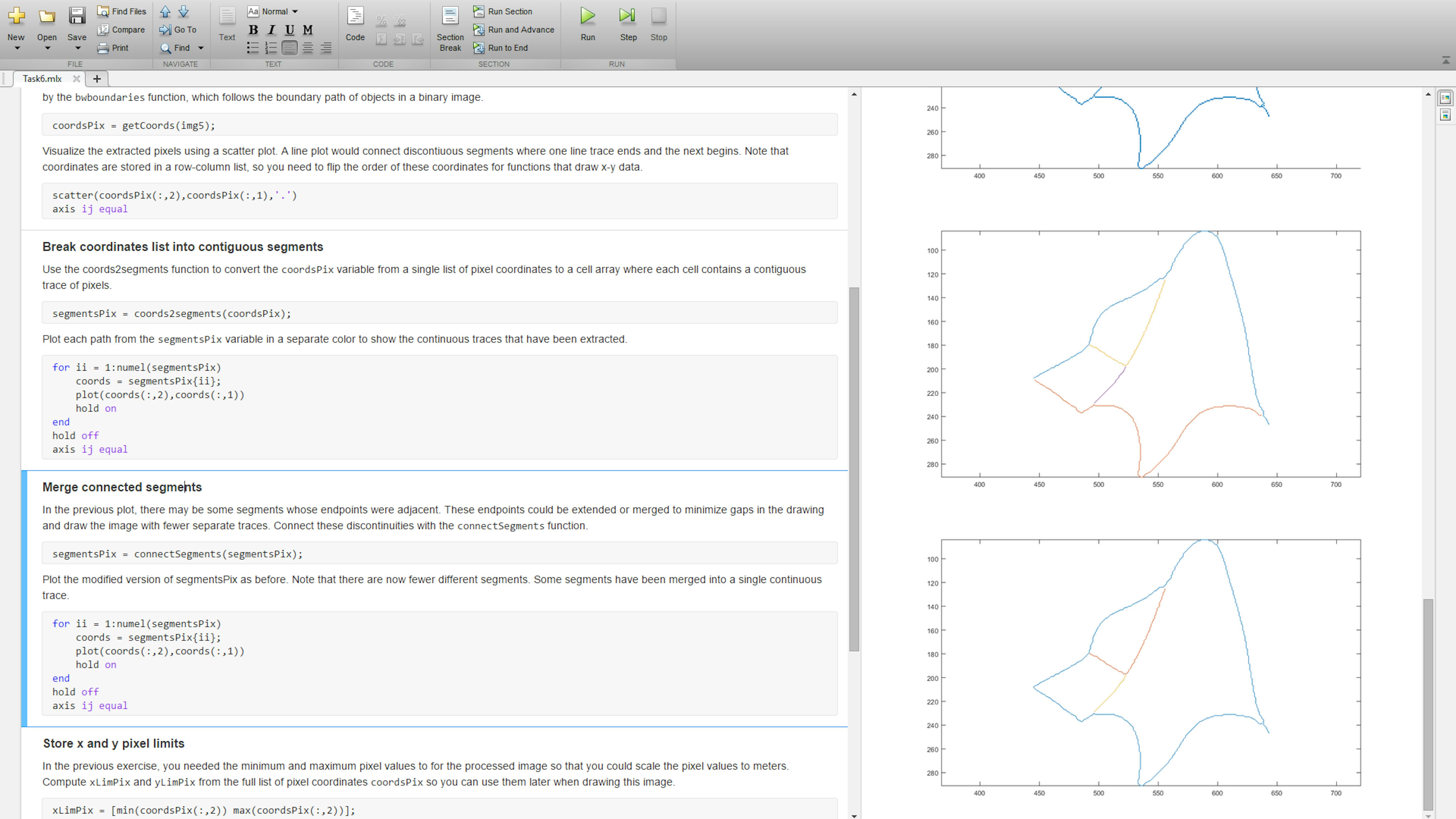
Also create new variables xLimPix and yLimPix as a quick way to store the maximum and minimum pixel positions for use when drawing the image on the whiteboard. Remember they are needed when estimating how to scale the image to fit on the whiteboard. Run the section of code with the heading Store x and y pixel limits .
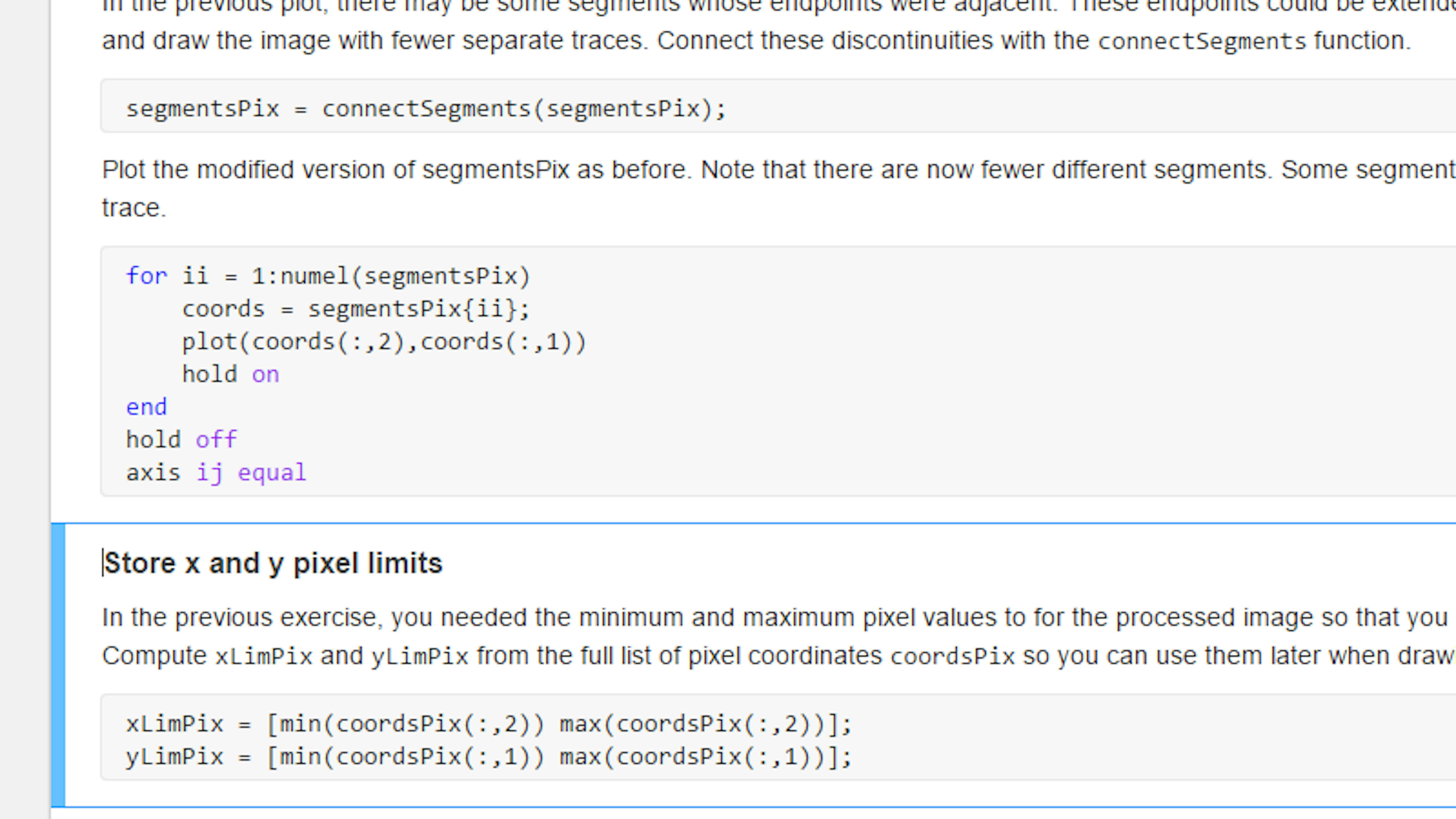
WRITE A FUNCTION TO CONVERT IMAGE TO PIXEL SEGMENTS
The code you've run up to now takes an image and generates groups of pixel positions. You can encapsulate all these steps in a function to easily perform them on any image. The function will return the segmentsPix , xLimPix , and yLimPix variables that you have computed. Create a new MATLAB function and call it imageToPixelSegments.m. Include the following code in the function and save it.
function [segmentsPix,xLimPix,yLimPix] = imageToPixelSegments(img)

% Extract line traces from image
img2 = ~imbinarize(rgb2gray(img), 'adaptive' , 'ForegroundPolarity' , 'dark' );
img3 = bwmorph(img2, 'clean' );
img4 = bwmorph(img3, 'thin' ,inf);

% Extract pixels in order
coordsPix = getCoords(img4);

% Break coordinates list into contiguous segments
segmentsPix = coords2segments(coordsPix);

% Clean data and merge connected segments
segmentsPix = connectSegments(segmentsPix);

% Store x and y pixel limits
xLimPix = [min(coordsPix(:,2)) max(coordsPix(:,2))];
yLimPix = [min(coordsPix(:,1)) max(coordsPix(:,1))];
Now check that the code in the imageToPixelSegments function behaves in the same way as the code you've executed so far. To do this, run the function and compare the result to the segmentsPix , xLimPix and yLimPix variables in your workspace. Run the section Test function imageToPixelSegments in Task6.mlx.
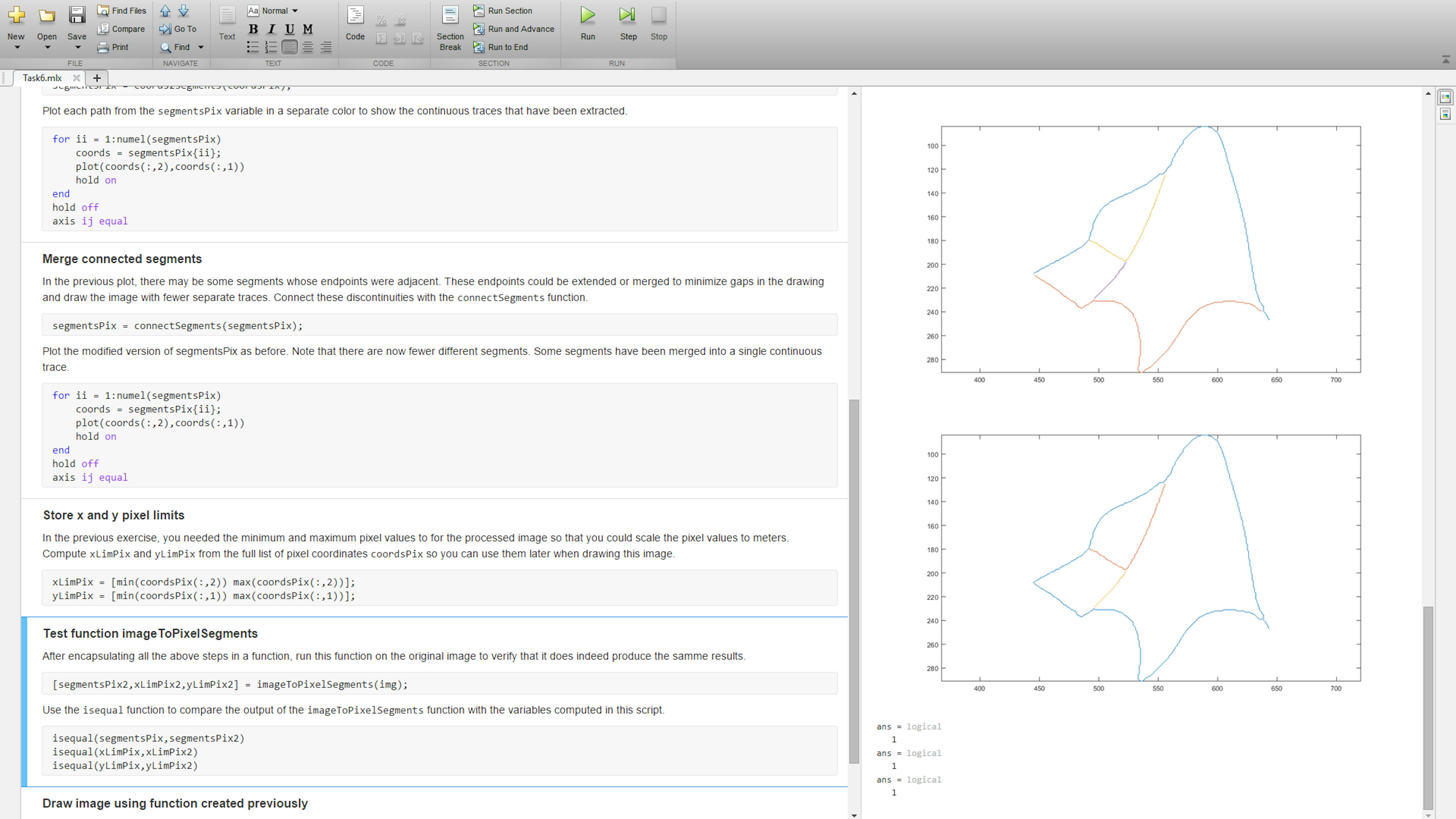
DRAW IMAGE ON WHITEBOARD
In the previous exercise, you wrote a function drawImageFromPix that takes a cell array of pixel paths and draws them on the whiteboard. Now you can call this function to recreate the MathWorks logo image on the whiteboard. Run the section of Task6.mlx with the heading Draw image using function previously created.
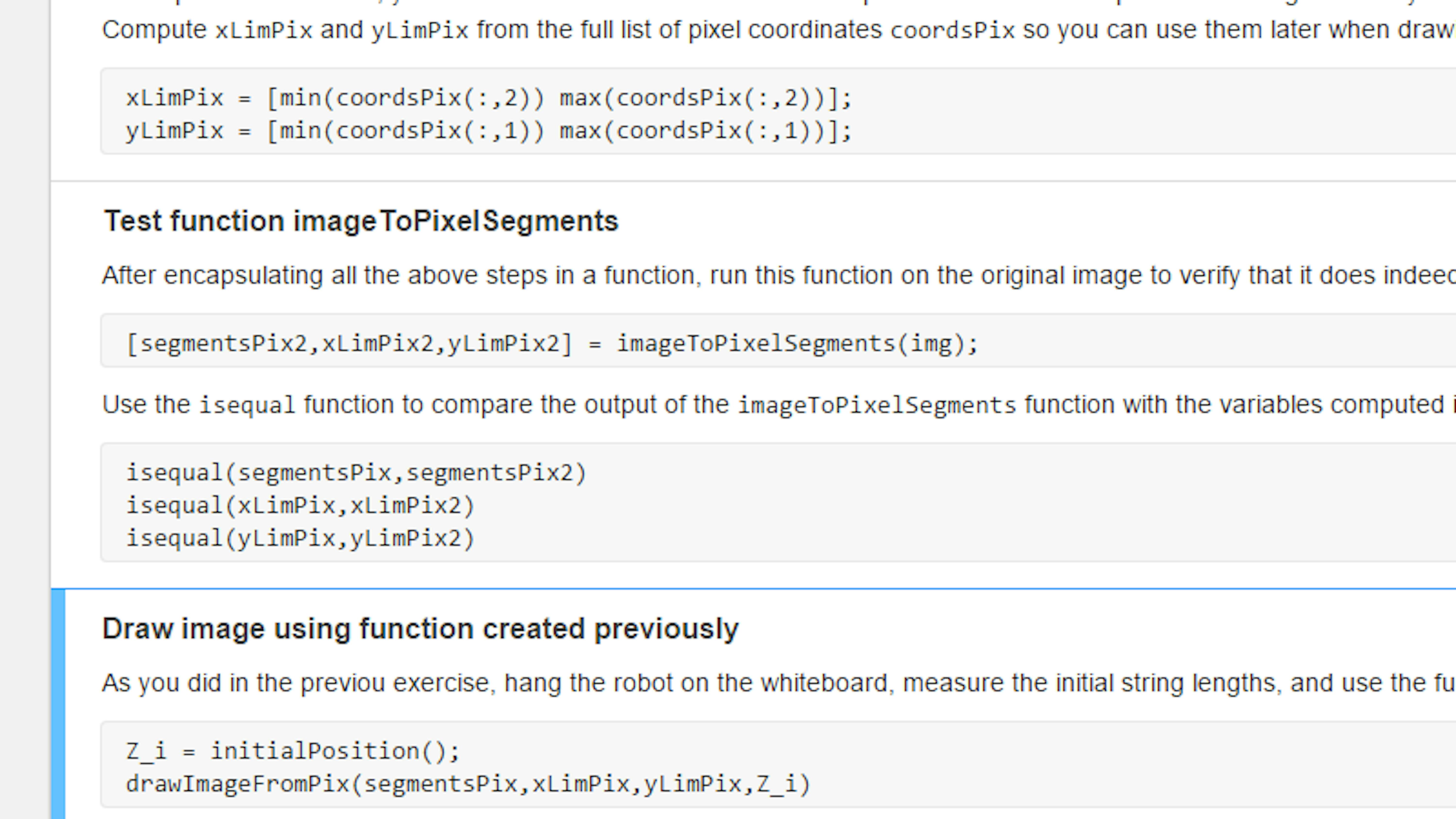
WRITE A MAIN SCRIPT TO RUN THE WHOLE WORKFLOW
To run an application with many steps, it is common to create a main script. This is a script that operates at the highest level and executes an entire workflow from start to finish. We can create a main script to perform all the tasks that you did in this exercise, relying on the functions you've created up to now.
Create a new empty MATLAB script. Add the following code and save the file as main6.m :
% Load image from file
img = imread( 'Images/MathWorksLogo.jpg' );

% Convert image to pixel segments
[segmentsPix,xLimPix,yLimPix] = imageToPixelSegments(img);

% Identify initial position on whiteboard
Z_i = initialPosition();

% Draw image
drawImageFromPix(segmentsPix,xLimPix,yLimPix,Z_i)
FILES
- Task6.mlx
- getCoords.m
- coords2segments.m
- connectSegments.m
- imageToPixelSegments.m
- main6.m
LEARN BY DOING
Use your understanding of recursive functions to write a new MATLAB function that will recursively compute the nth value of the Fibonacci sequence. Recall that the nth Fibonacci number is the sum of the two previous Fibonacci numbers and the first two are 0 and 1. Your recursive function should have two stopping conditions (for when n = 1 or n = 2). For all other cases, your function should recursively call itself twice.
In this exercise, you are loading an image from a file, processing it, and then drawing it immediately. You may instead want to just do the processing on your images, preview the extracted line traces, and store this pixel data in a MAT-file to load and draw later. Write a function that will do this. When saving the data to a MAT-file, you will need to specify a filename. There are two ways you can specify it. One is to choose the name based on the filename of the image. Use matlab.lang.makeValidName to ensure the name is valid. The second option is to prompt the user for a name using the uiputfile dialog.
In your main6.m script, you have hardcoded the name of the image file to process. To make the script more user-friendly and allow you to draw different types of images, you may want to change this so that the user can interactively select which image to draw. Modify the beginning of main6.m so that it prompts user to select a file, rather than defining it in the code. You can use the uigetfile dialog for this.
Exercise 7:
4.7 Capture and draw live images
By now, your drawing robot is pretty capable. It can take any image file and reproduce the image on a whiteboard. All of this is automated in code. But there are still some manual steps that involve taking the image, transferring the file to your computer, and specifying that file as the one you want to draw. In this exercise, you'll automate these steps as well by using a webcam to capture the image and bring it directly into MATLAB to analyze and draw with the robot.
In this exercise, you will learn to:
- Connect to a webcam
- Update a main script
CONNECT TO WEBCAM
In addition to Arduino devices, MATLAB can talk to many other types of hardware. To acquire images directly into MATLAB, you can use a USB webcam. MATLAB's webcam interface can connect to webcams, preview what they see, and take snapshots that bring the current image directly into MATLAB. This functionality requires MATLAB Support Package for USB Webcams , which you should have installed when setting up all your MATLAB and Simulink software. If you have not yet installed the support package, install it now. Find the USB webcam that is included in the kit and connect it to your computer. Open the live script Task7.mlx .
>> edit Task7
To identify the webcam in MATLAB and connect to it, run the section of code under the heading Connect to webcam .
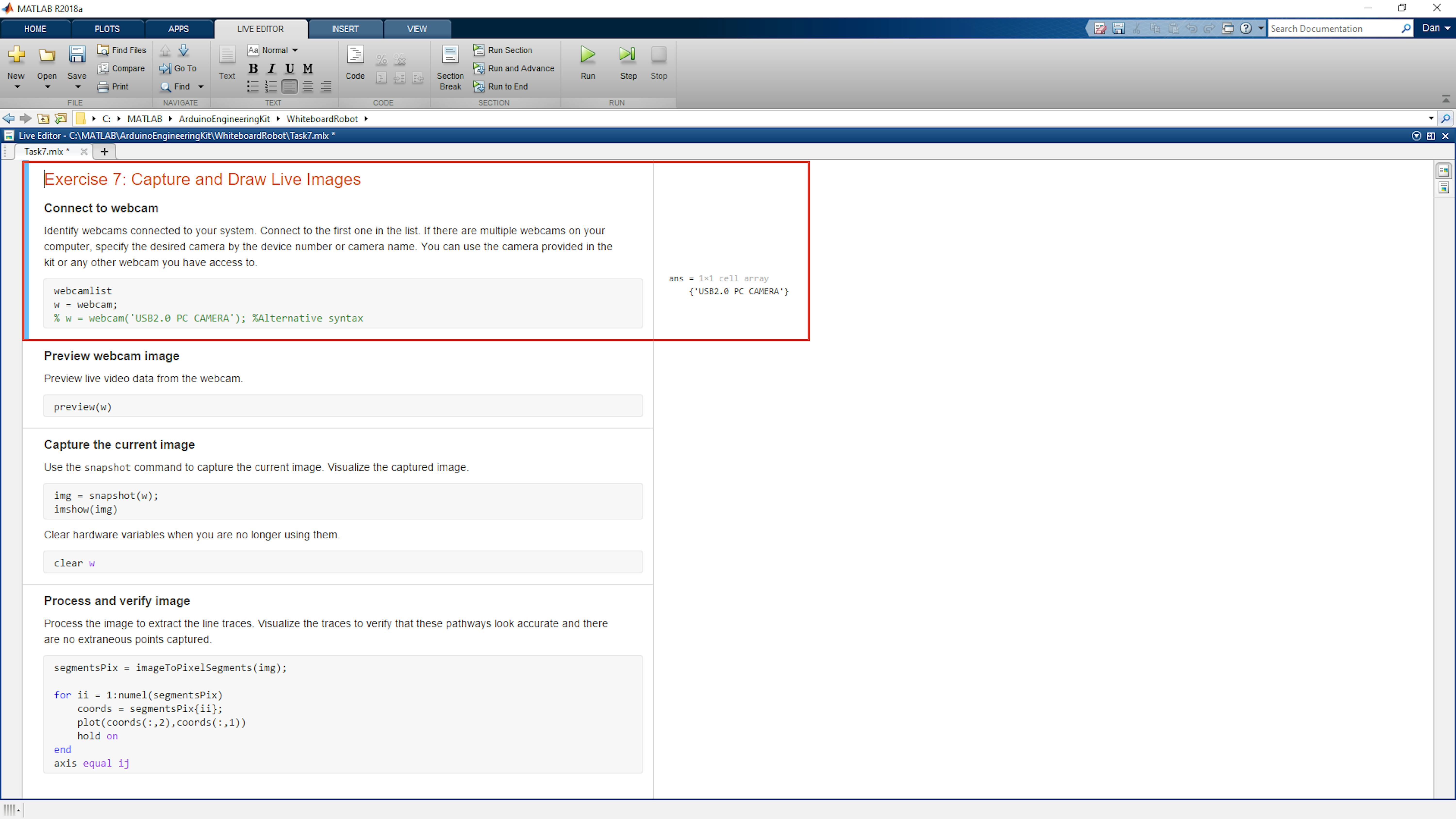
PREVIEW WEBCAM IMAGE
Preview the webcam image in MATLAB by running the section of code with the heading Preview webcam image.
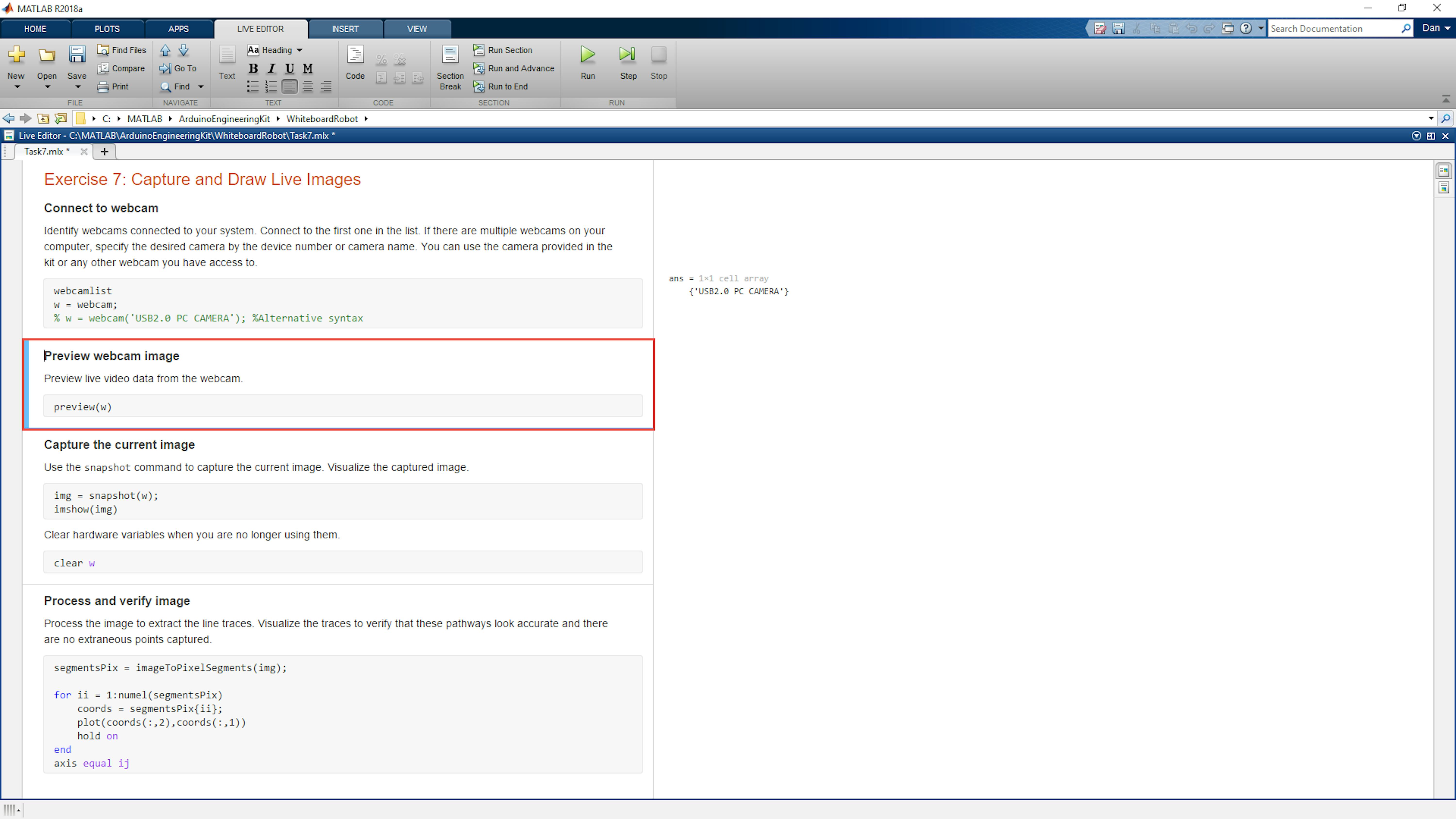
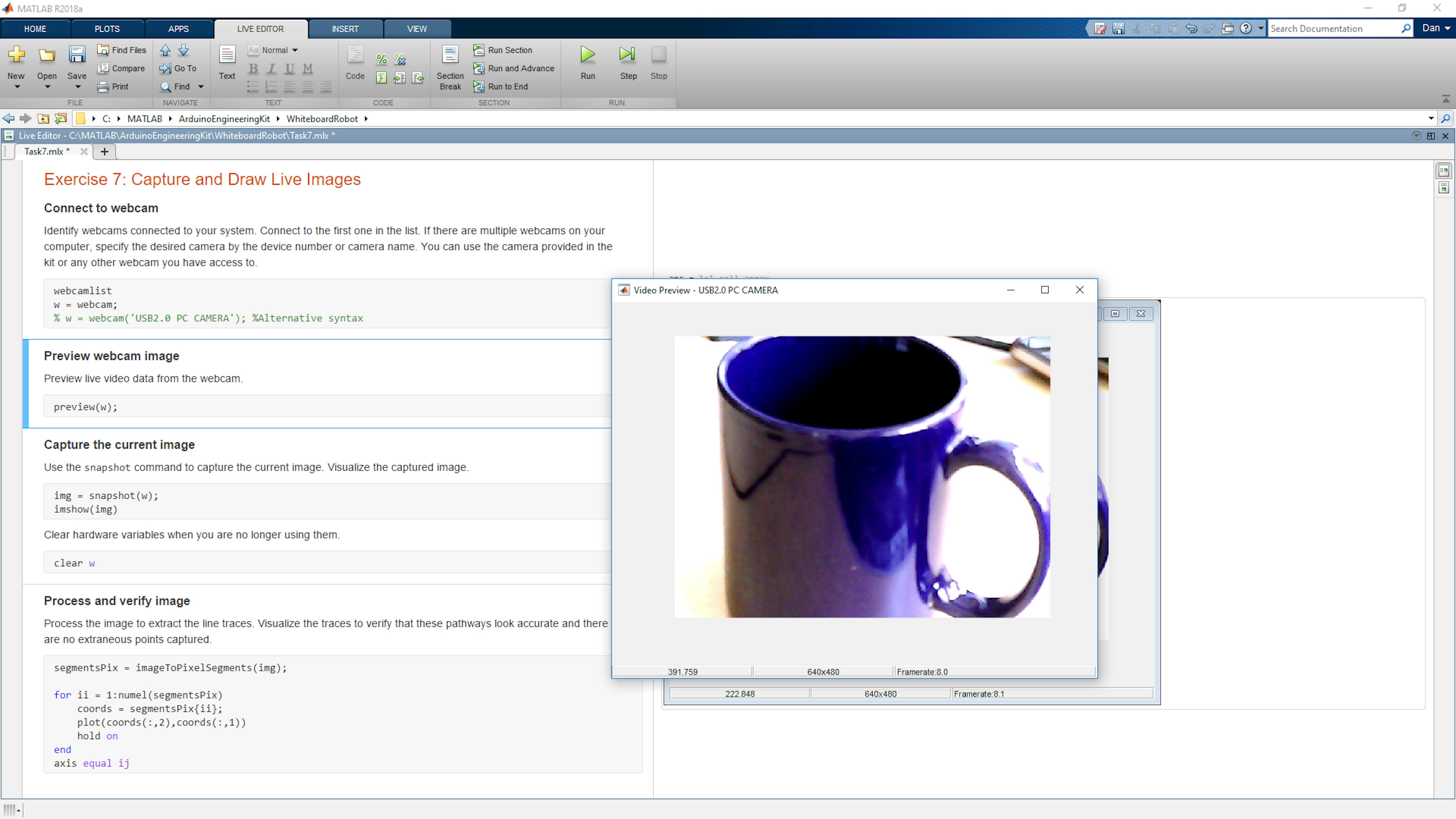
Move the webcam around to make sure it can get a clear view of images in view.
CAPTURE CURRENT IMAGE
Using a black marker, create a simple line drawing on your whiteboard that you'd like your robot to recreate. Aim the camera at the whiteboard and check the preview window to make sure that the drawing is clear, there is nothing else in the view of the camera, and there is no glare or uneven lighting on the whiteboard. Alternatively, you can use a pen drawing on a white piece of paper.
Capture an image of the drawing. Run the section of code in Task7.mlx with the heading Capture the current image.
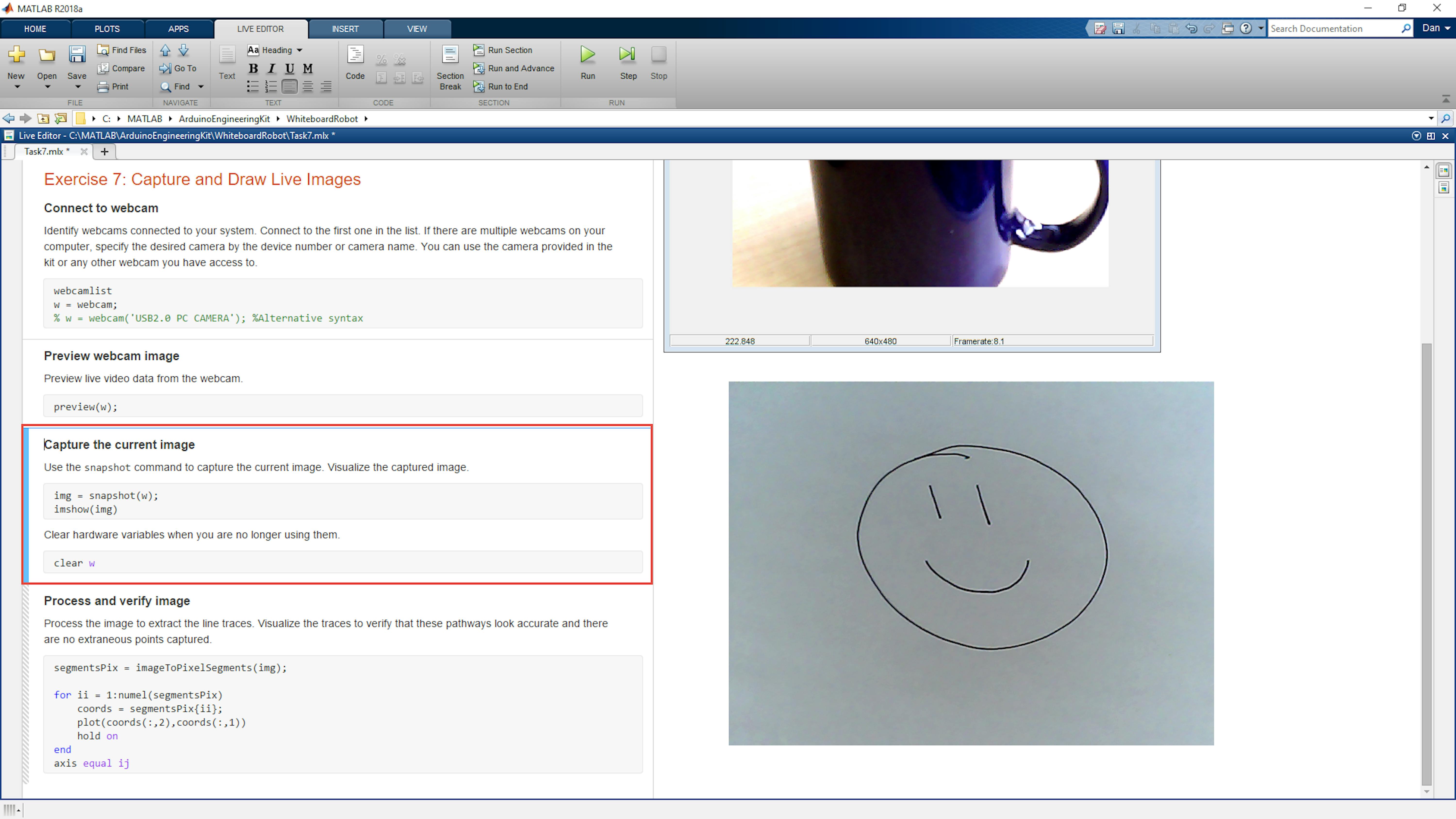
PROCESS AND VERIFY IMAGE
To make sure that your image will draw correctly with the robot, run your image processing function imageToPixelSegments , and check that the extracted paths in the image are as expected. Run the section of Task7.mlx under the heading Process and verify image. If the processed version does not look correct, take a new image and try again.
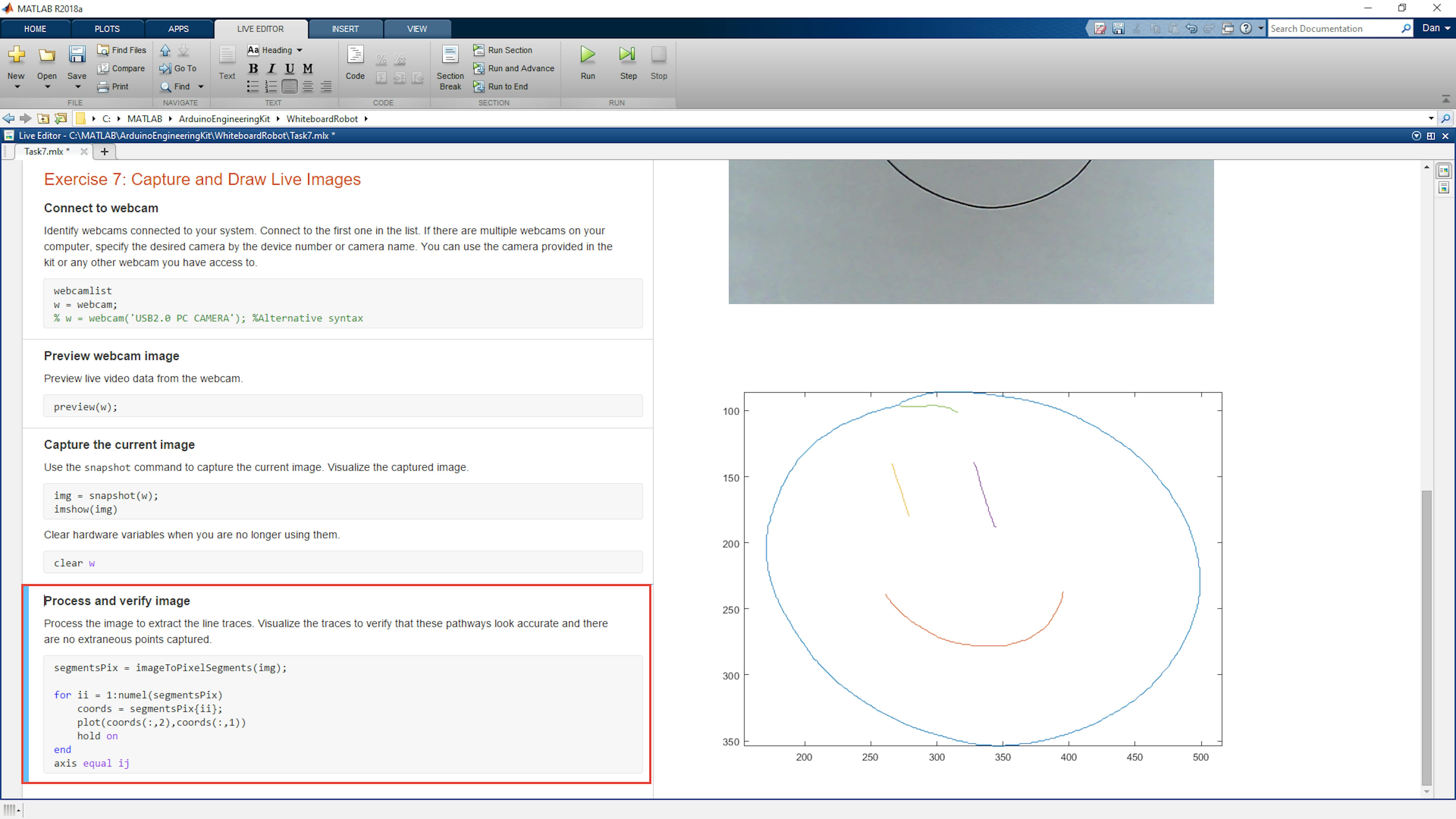
UPDATE MAIN SCRIPT FOR LIVE IMAGES
In the previous exercise, you created a main script to run the full application altogether. That script loaded the desired image from a file. Now, you'll modify that script so it can get the image from the camera. Open the file main6.m. Save a new version of the file as main7.m. Delete the first line of code from main6.m, which loads the image from the file. Replace it with code that will connect to the webcam, preview the image, and wait until you strike a key before taking a snapshot of the current image and continuing with the script. The full main7.m script should look as follows:
% Capture image from webcam
	w = webcam;
	preview(w)
	pause
	img = snapshot(w);
	clear w

% Convert image to pixel segments
	[segmentsPix,xLimPix,yLimPix] = imageToPixelSegments(img);

% Identify initial position on whiteboard
	Z_i = initialPosition();

% Draw image
	drawImageFromPix(segmentsPix,xLimPix,yLimPix,Z_i)
RUN MAIN SCRIPT TO DRAW AN IMAGE CAPTURED LIVE
Now try it out with your robot. At the MATLAB command prompt, run your main script.
>> main7
A webcam preview window will open. Aim your camera at a white region of the whiteboard with a simple line drawing on it. Make sure nothing else is in the frame of the image and there is no glare or color variation across the image. Strike any key in MATLAB to continue. The robot will scale the captured image to the full whiteboard and attempt to reproduce it.
FILES
- Task7.mlx
- main7.m
LEARN BY DOING
At the end of this task you should be able to acquire an image from a USB webcam and immediately draw it with your robot. Another possible application for the webcam might be to acquire a whole set of images of whiteboard drawings to reproduce later with the robot. Starting with the code you already have, create a script that can acquire a webcam image, prompt the user for a filename, and save the image with that name. Refer to the functions uiputfile and imwrite for help with these tasks.
4.8 Lessons learned
In this chapter you were introduced to these following topics:
APPLY TRIGONOMETRIC THEORY TO CONTROL THE MOVEMENTS OF THE ROBOT.
In this project you have learned how to decompose movements through trigonometry to calculate the distances that allow the robot to draw on the whiteboard. As well, you combined the trigonometry with motion equations to move the robot to some specific points in your whiteboard. You did it using MATLAB scripts and searching the information of the motors in its datasheets.
KNOWING THE LIMITATIONS OF THE ROBOT MOVEMENTS
After knowing how to program the robot movements, you have learned where the limits are. Why the robot cannot arrive to some positions and what are the allowed areas to draw with it.
IMAGE PROCESSING
You also have learned how to processing a image to get the needed data to draw it in the white board. To do it, you have learned how to apply some image filters, how to get the lines of the draw, how to convert the pixels to meters and how to build segments to create the trajectory that the robot will follow.
4.9 Final challenge
Throughout this project, you've drawn images on the whiteboard using only one marker. However, your drawing robot can hold two markers. It would be nice if you could draw images that have more than one color. How might you go about doing this?
The simplest approach would be to alternate colors for each line segment. Another approach might be to group the objects in the image based on how close they are to one another and draw each group the same color. Or combine two different images and draw each in a different color. Maybe you could identify line traces of different colors within a single image and draw them separately. How would you do that using image processing? Try using the Color Thresholder app from Image Processing Toolbox. Your final challenge is to come up with an interesting way to create drawings that use multiple marker colors. You can try one of the ideas listed or come up with your own. Implement the solution in MATLAB, and then draw a multi-color image with your robot.