
Mobile Rover
Introduction
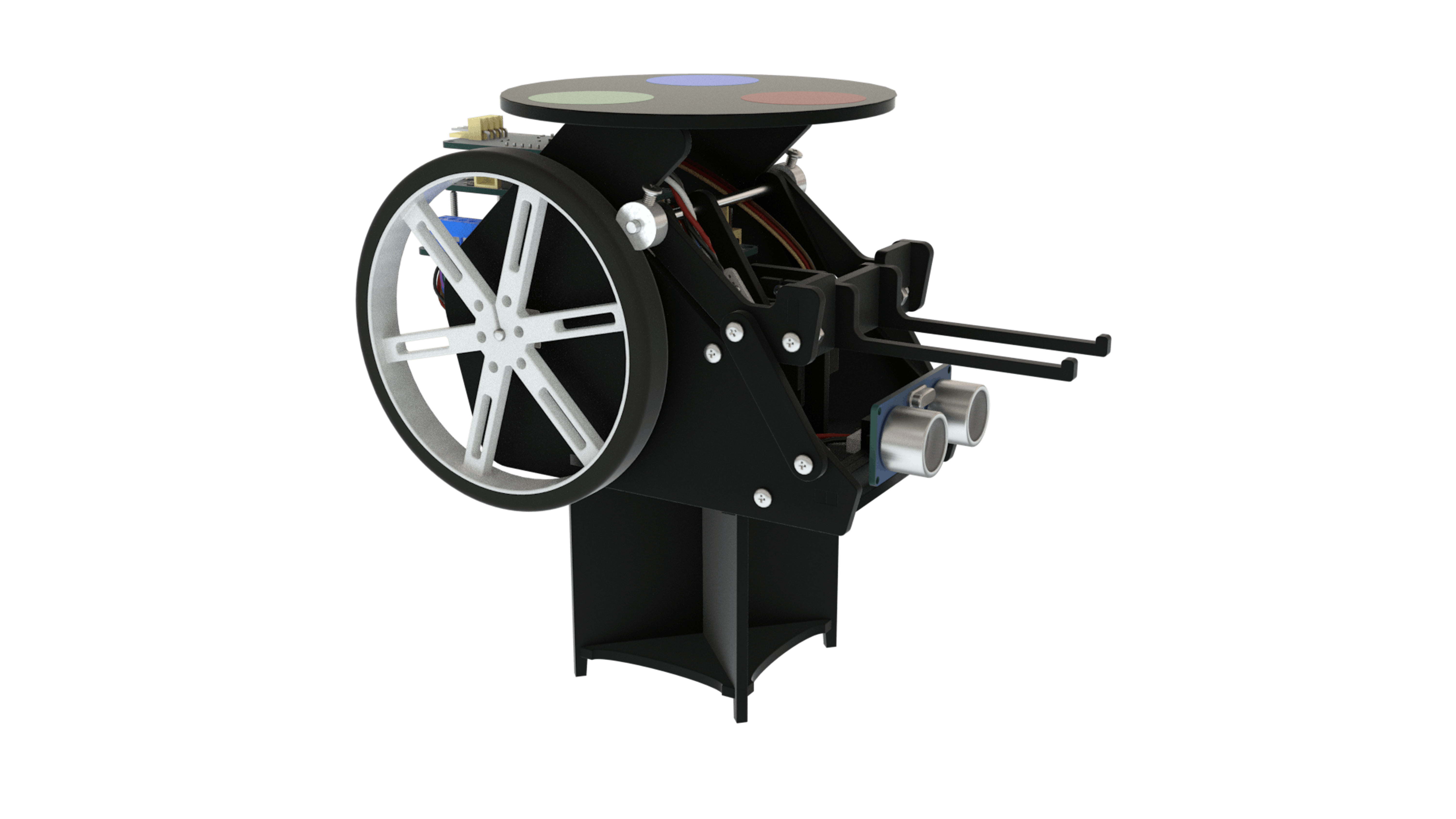
The mobile rover project consists of a programmable robot that can communicate with MATLAB over Wi-Fi to perform operations using an image processing algorithm. The rover is controlled by an Arduino MKR1000, the Arduino MKR Motor Carrier, two DC motors with encoders, a micro-servo motor, and a couple of sensors. On top of the rover, you will install a color-coded sticker that will serve as a marker to assist the image processing algorithm that uses a webcam to detect the location and orientation of the robot.
In this project, you will program the mobile rover to perform a variety of tasks, such as following paths, moving objects with the forklift, and avoiding obstacles. You will learn important robotics concepts including how differential drive robots work and how to simulate their behaviour, control their position or speed, and perform localization. After completing the project, you will have the knowledge to develop and program your own robots to intelligently travel around and perform all kinds of fun tasks.
By the time you are ready to start with the coding, you should have assembled the rover following the instructions you can find at:
In the exercises that make up this project, you will learn to:
- Exercise 1: Control the rover and forklift from MATLAB.
- Exercise 2: Use kinematic equations to simulate the rover motion and perform open-loop control.
- Exercise 3: Perform closed-loop control of the rover.
- Exercise 4: Use states to a) program your rover to follow sequence and b) eliminate steady-state error and overshoot of your closed-loop controller.
- Exercise 5: Localize the rover using image processing.
- Exercise 6: Control the rover and forklift to pick up the target and drop it off.
- Exercise 7: Enable Wi-Fi communication between rover and MATLAB.
Note: The default wire length of the DC motor with encoder is necessary for the drawing robot. It is advised not to shorten the wire length for the Mobile Rover
EXERCISE 1:
5.1 Control the Rover and Forklift from Matlab
The mini mobile rover is a differential drive robot that has separate DC motors controlling each of its wheels. You can control the direction of travel by varying the speed of each wheel without the need for any separate steering mechanism. In this exercise, you will learn how to drive the rover and operate the forklift using MATLAB.
In this exercise, you will learn to:
- Control basic movement of a differential drive robot.
- Connect MATLAB to the rover.
- Drive the rover in a straight line.
- Drive the rover in circles.
- Control the forklift of the rover.
HOW TO COMMUNICATE WITH THE ROVER
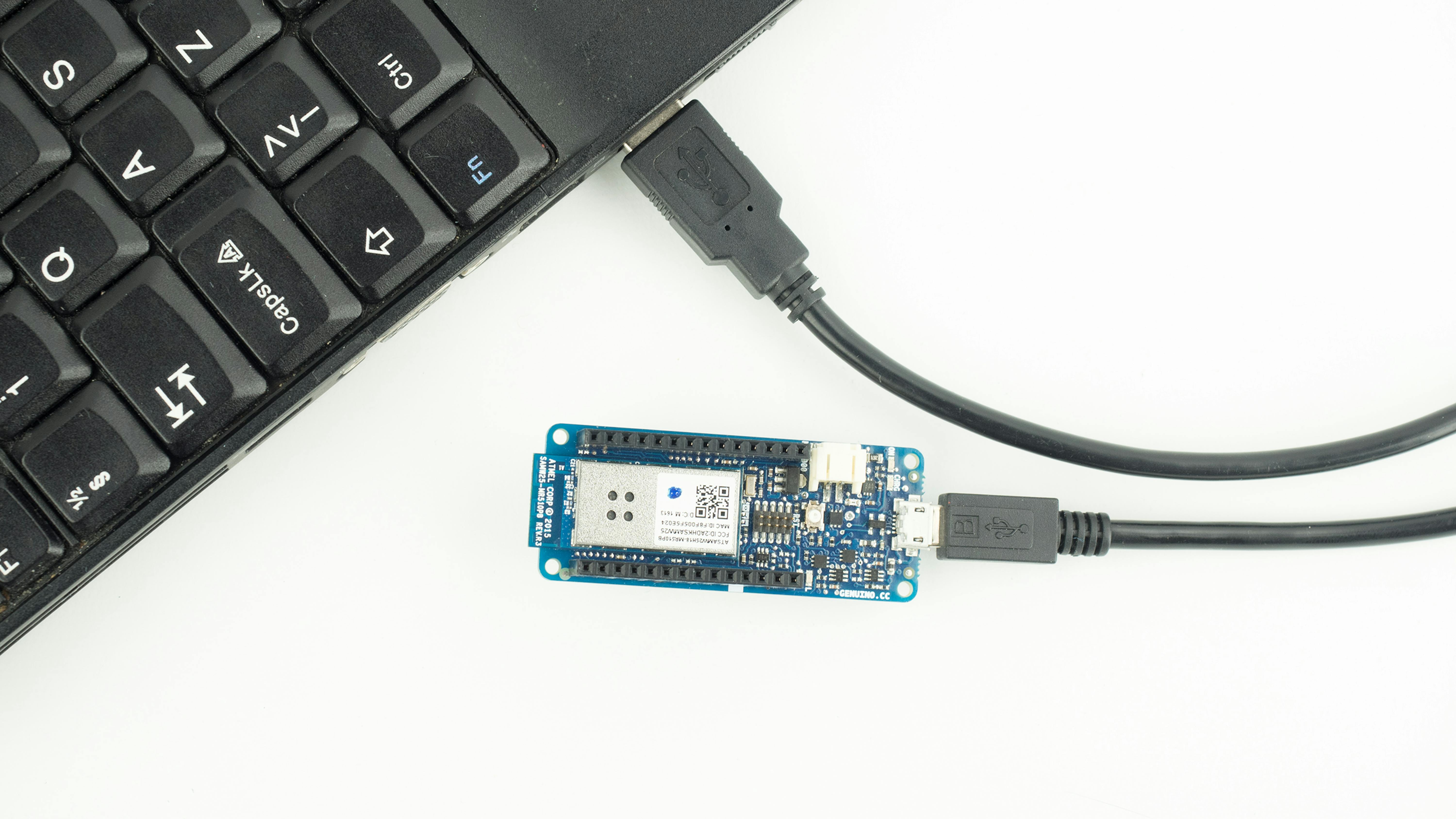
Let's begin by connecting the Arduino MKR1000 to your computer using the USB cable:
To communicate between MATLAB and Arduino, you need to know the port number your Arduino is connected to. You can determine this using the steps described in section 2.1.3 Working with Digital Outputs in "2.1 Arduino Getting Started". Remember that the port names differ between operating systems; in other words, they are different for Windows (where they are named COM## with the ## being a unique numeric identifier), OSX (/dev/tty.usbmodem##), and Linux (/dev/ttyACM##).
Once you know the port number , enter the following commands with the appropriate port number to create (a) an Arduino object with the necessary libraries and (b) a separate object for the motor carrier:
>> a = arduino(' COMX', 'MKR1000', 'Libraries', 'Arduino/MKRMotorCarrier');>> carrier = addon(a,'Arduino/MKRMotorCarrier');CONTROL THE ROVER FROM MATLAB
Drive in a straight line
You probably know intuitively that the rover will travel in a straight line if both wheels spin at the same speed and in the same direction. Let's spin the rover's DC motors at the same speed and observe whether it goes in straight line as expected. Enter the following commands to connect the DC motors to MATLAB:
>> dcmLeft = dcmotor(carrier,4);>> dcmRight = dcmotor(carrier,3);Now specify that you want the DC motors to spin at 25% of the maximum speed:
>> dcmLeft.DutyCycle = 0.25;>> dcmRight.DutyCycle = 0.25;Once you've specified how fast the motors must spin, the next step is to spin them! Enter the following commands to run the motors for 10 seconds at this speed:
>> start(dcmLeft)>> start(dcmRight)>> pause(10)>> stop(dcmLeft)>> stop(dcmRight)Measure how far the rover moved when using these commands. Since the information coming from the encoders attached to each one of the DC motors is not being read yet, there is no way to ensure that the rover will either move completely straight (there might be slight differences in behavior between the motors), or that it will move the same distance each time the program is executed (as time goes by, the batteries will have less and less charge and will behave differently).
Drive in a circle
If you were asked how to drive the rover in a circle, your answer might be a) to spin one wheel but not the other, or b) spin both wheels with the same speed but in opposite directions.
Both answers are correct, though the way the rover will move will differ. Let's analyze the first case:
Spin one wheel but not the other. Try the following commands with the rover:
>> dcmLeft.DutyCycle = 0;>> dcmRight.DutyCycle = 0.25;>> start(dcmLeft)>> start(dcmRight)>> pause(10)>> stop(dcmLeft)>> stop(dcmRight)You should observe that the rover spins in a circle around its left wheel.
The other case required you to spin both wheels with the same speed but opposite directions. Let's try spinning the wheels with equal and opposite speed by running the following code in MATLAB:
>> dcmLeft.DutyCycle = -0.25;>> dcmRight.DutyCycle = 0.25;>> start(dcmLeft)>> start(dcmRight)>> pause(10)>> stop(dcmLeft)>> stop(dcmRight)You should observe that the rover spins in a circle about its center.
CONTROL THE FORKLIFT OF THE ROVER
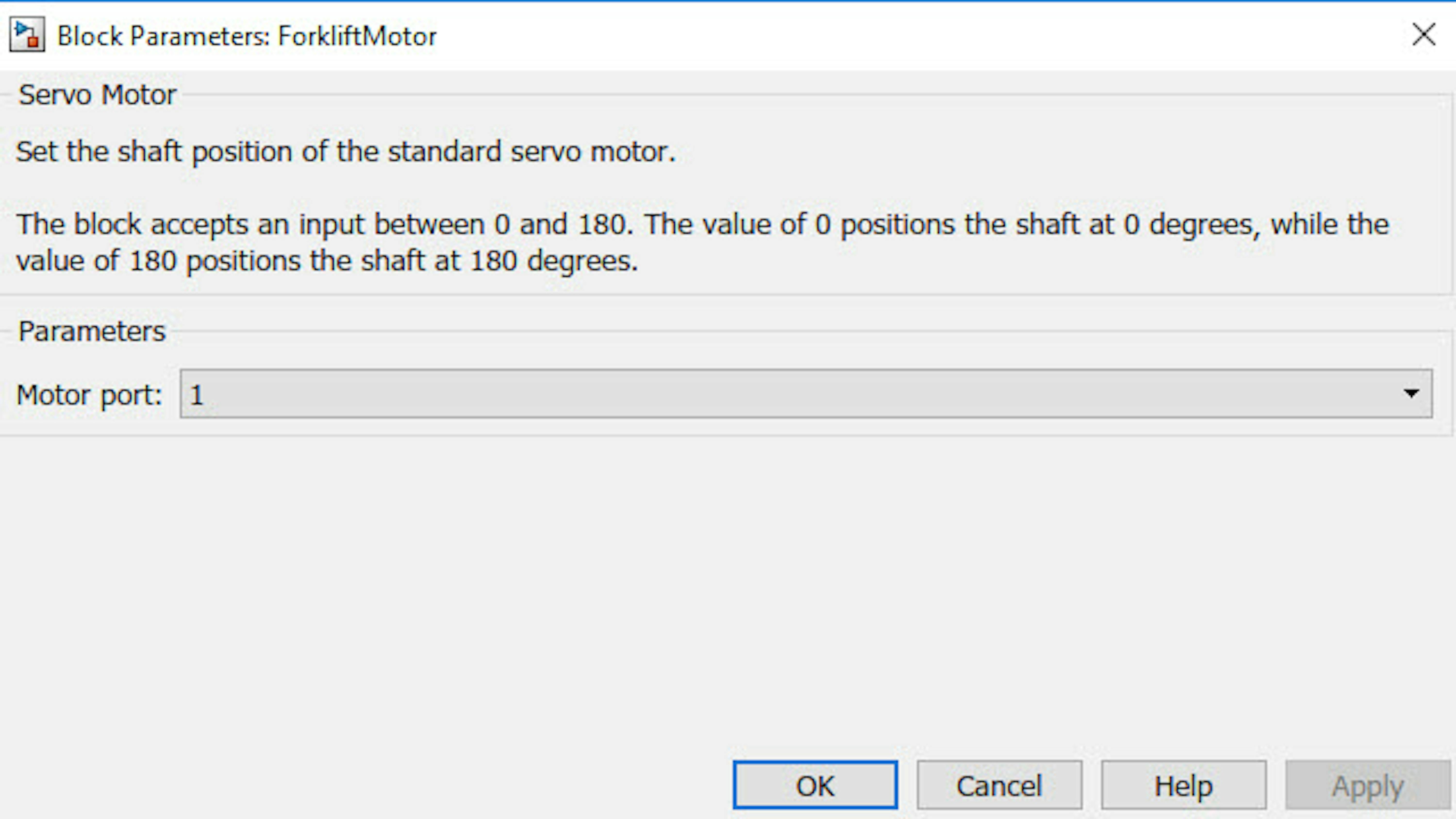
The rover's forklift is controlled by a standard servo motor connected to the MKR motor carrier board; this means you can control the angle at which the motor will turn. Typically, standard servos can turn between 0 and 180 degrees, but there might be other types.
Note: Arduino Engineering Kit only provides standard servo motors.
In this section, first you will move the servo to the "Down" position, which corresponds to an angle of zero degrees. You will use the writePosition(s,0); statement shown in the code below for this. Then you will move the servo to the "Up" position, which corresponds to an angle of 125 degrees on the actual servo motor. In the second input of the writePosition function, 0 represents the minimum position possible, which is zero degrees for standard servo motors, and 1 represents the maximum position possible, which is 180 degrees. Enter the following commands to connect to the servo and move the forklift between the Up and Down positions:
>> s = servo(carrier,1);>> writePosition(s,0)>> pause(5)>> writePosition(s,0.7)REVIEW/SUMMARY
-
We have seen how to drive the rover in a straight line and in circles.
-
We have seen how to control the forklift, which will be used in later exercises to lift the target.
LEARN BY DOING
-
Drive the rover in a circle of different radius by sending different speeds to both wheels.
-
Drive the rover in a sequence: move forward, then turn left 90 degrees in place, and then move forward again.
EXERCISE 2
5.2 Simulating Rover kinematics and open loop control
In Exercise 1, you learned how to make the rover drive in a straight line and in circles. However, to move the rover along more complex paths you need to understand the underlying kinematic equations that relate the speed of each wheel to the rover velocity and direction of travel. In this lesson, you will learn the basic kinematic equations behind differential drive robots and how Simulink can help you visualize and simulate the rover's movement for various inputs. You will then apply what you learned through these simulations to control the rover in the real world.
In this exercise, you will learn to:
- Understand kinematic equations of the rover.
- Simulate the rover using kinematic equations.
- Model and simulate rover movement using Simulink.
- Perform open-loop control of the rover.
- Use Simulink models to control the actual rover.
KINEMATICS OF THE ROVER
The following diagram shows the basic kinematics of the rover (or any differential drive robot):

The diagram introduces a few important parameters associated with differential drive robots, including radius of rotation (R), rate of rotation (ωl), instantaneous center of curvature (ICC), wheel velocities (vl, vr), rover length (L) and forward velocity (v). If you want to learn more about the concepts presented in this diagram, please refer to this page.
Let's begin by focusing on rate of rotation and forward velocity.
Rate of rotation: $\omega =\frac{v_{r}-v_{l}}{L}$
Forward velocity: $v=\frac{v_{r}+v_{l}}{2}$
Wheel velocities (vl , vr) can be calculated based on wheel radius (r) and rotational speeds (ωl, ωr):
$v_{l}= \omega _{l} \cdot r$
$v_{r}= \omega _{r} \cdot r$
Plugging these values into the previous equations yields:
$\omega =\frac{r\cdot \left( \omega _{r}- \omega _{l} \right) }{L}$
$v=\frac{r\cdot \left( \omega _{r}+ \omega _{l} \right) }{2}$
Rearranging these equations:
$\omega _{r}+ \omega _{l}=\frac{2v}{r}$
$\omega _{r}- \omega _{l}=\frac{L \omega }{r}$
Solving for ωr and ωl:
$\omega _{r}=\frac{v+ \left( \frac{L}{2} \right) \omega }{r}$
$\omega _{l}=\frac{v- \left( \frac{L}{2} \right) \omega }{r}$
In Matrix notation:
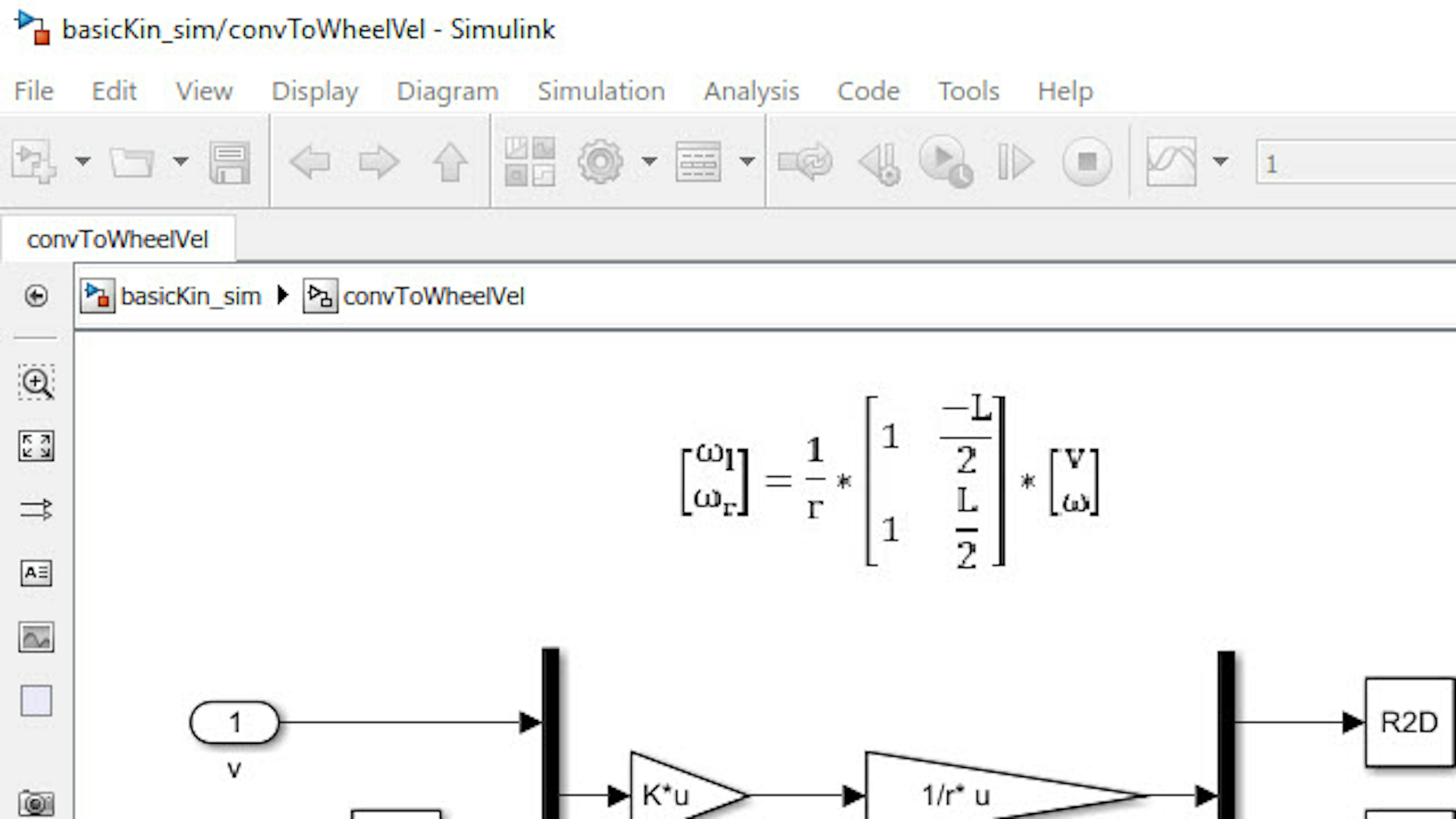
$\left[ \begin{matrix} \omega _{l}\\ \omega _{r}\\ \end{matrix} \right] =\frac{1}{r}\cdot \left[ \begin{matrix} 1 & \frac{-L}{2}\\ 1 & \frac{L}{2}\\ \end{matrix} \right] \cdot \left[ \begin{matrix} v\\ \omega \\ \end{matrix} \right]$
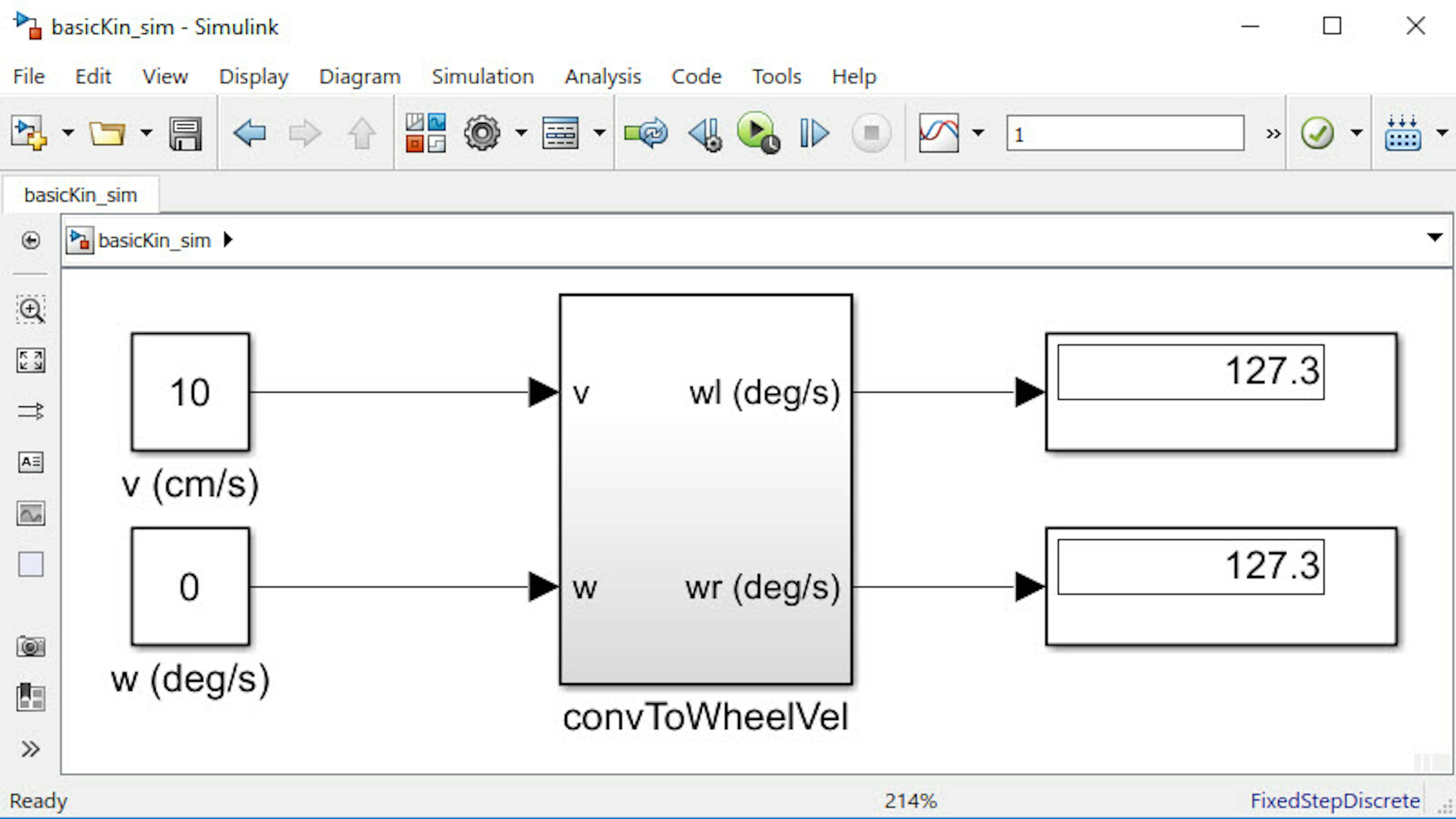
For our rover, L = 8.8 cm and r = 4.5 cm. Using these values and the above equations, let's calculate how fast to spin each wheel to move the rover at a desired forward velocity and rate of rotation. Let's look at two simple scenarios:
- Drive rover straight forward at 10 cm/s (v = 10 cm/s, ω = 0 deg/s) ωr = ωl = 127.3 deg/s (includes unit conversions)
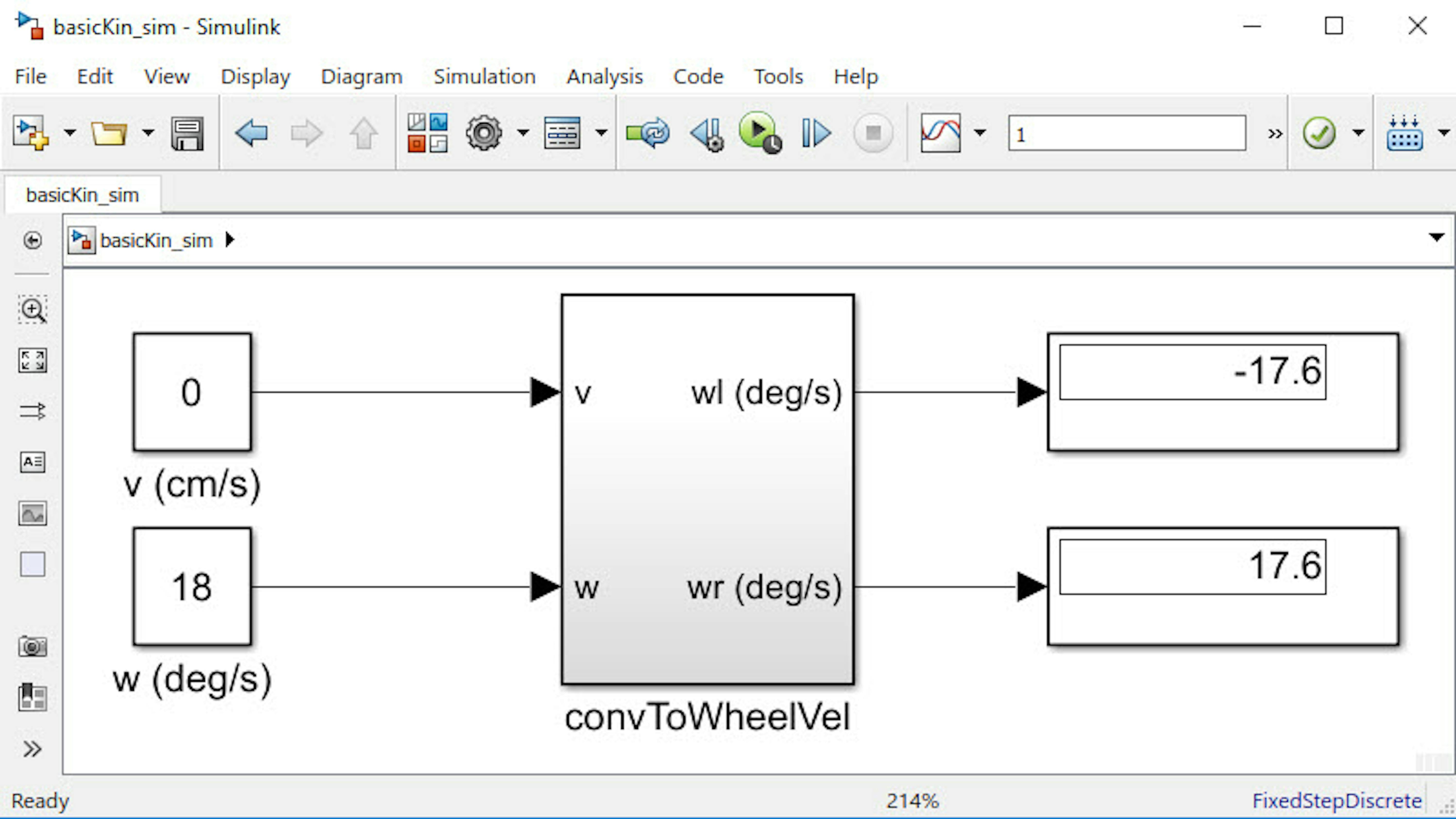
- Spin rover 180 deg in 10 seconds with zero forward velocity (v = 0 cm/s, ω = 18 deg/s)
$\omega _{r} = 17.6 deg/s$, $\omega _{l} = -17.6 deg/s$ (includes unit conversions)
IMPLEMENTING EQUATIONS IN SIMULINK
The goal of this example is to guide you into implementing the above-presented equations, using Simulink, that can then be used to drive the rover. We have prepared a model in which a series of blocks are connected to each other; they perform the matrix operations shown in the equations above and compute the angular speeds for each one of the motors (ωr and ωrl) given a desired linear and angular speed of the whole rover. Open the model by typing the following command in MATLAB:
>> basicKin_sim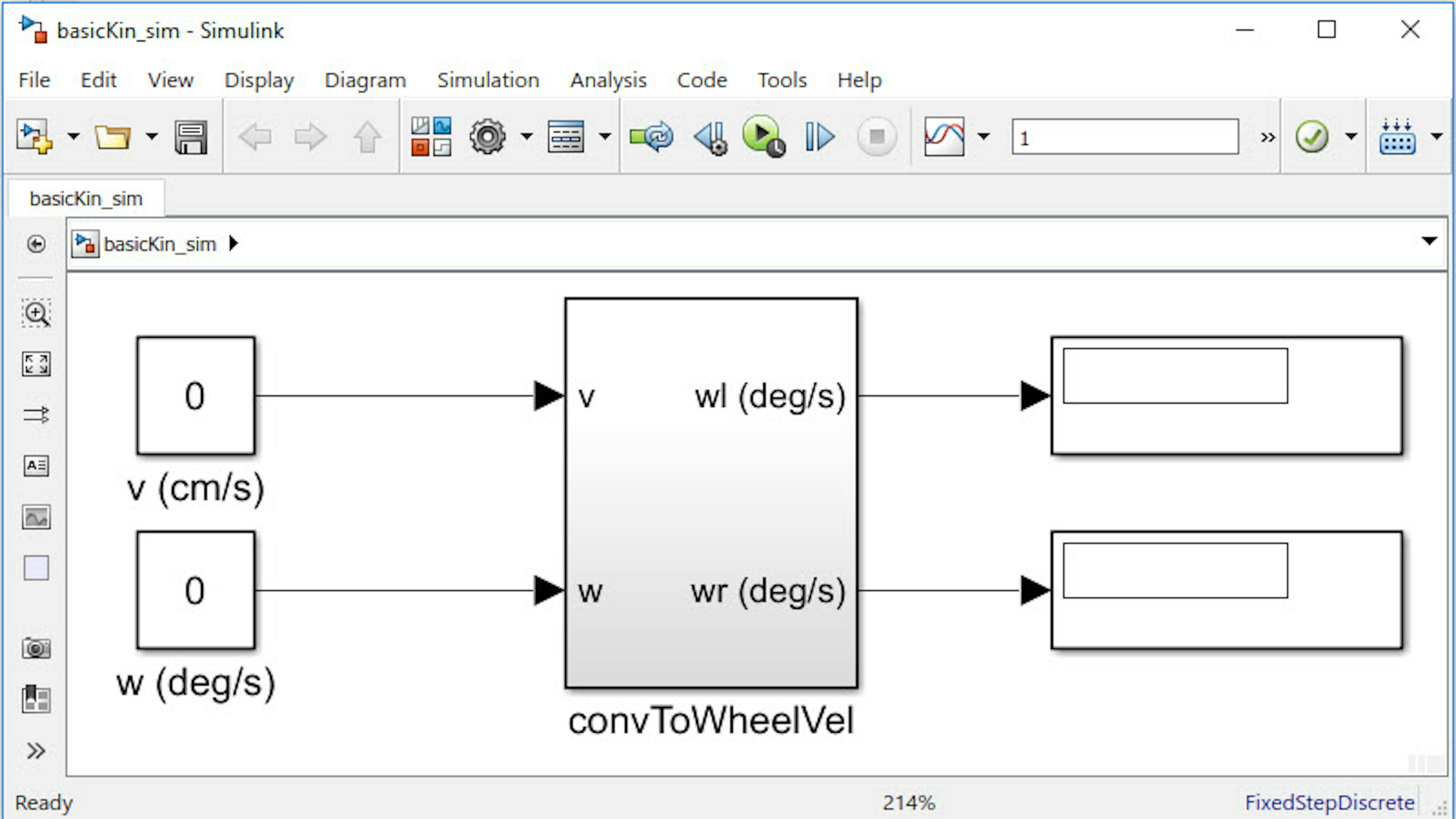
The blocks on the left are constant blocks where you can specify desired rover velocity and rate of rotation. The blocks on the right are display blocks and will show the resulting ωl and ωr values.
But before looking at the convToWheelVel subsystem, note that L, r, and TS were defined in the Workspace.
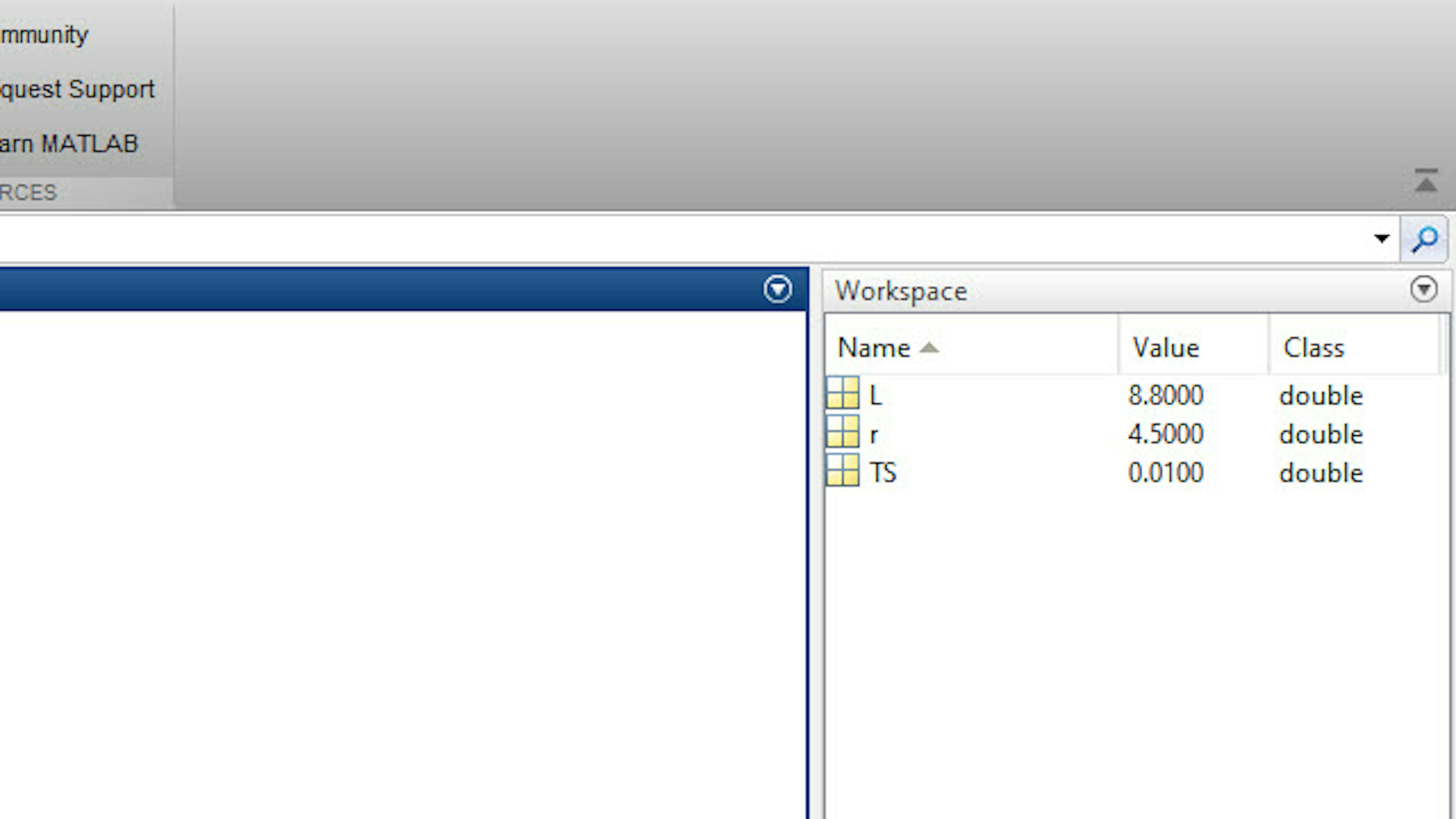
Simulink has the concept of model callbacks, and they are used to call MATLAB scripts or functions at different times. This model uses the callback PostLoadFcn to call a MATLAB script right after loading the Simulink model into the memory. The script being called here is paramsBasicKinematics, and these variables (L,r,and TS) are defined as constant values in this script.
L and r are dimensions of our rover, and TS is the sample time of the model. Sample time is a parameter that indicates when outputs of the Simulink model should be produced and, if appropriate, when to update blocks during simulation.
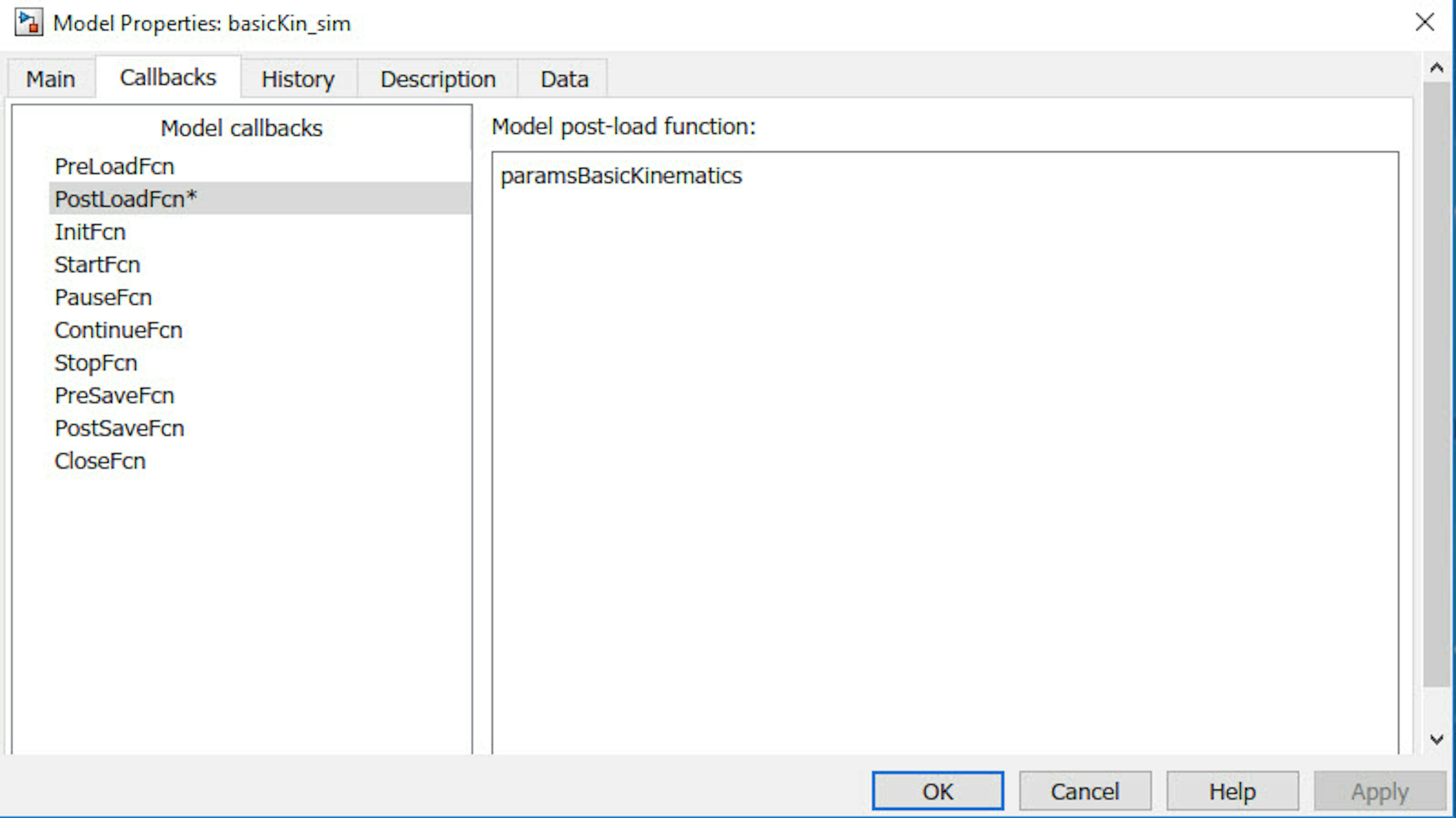
You can view the model callbacks by selecting File > Model Properties > Model Properties from the Simulink toolbar. Click Callbacks in the Model Properties window that popped up as shown below.
Now let's open the convToWheelVel subsystem by double-clicking it.
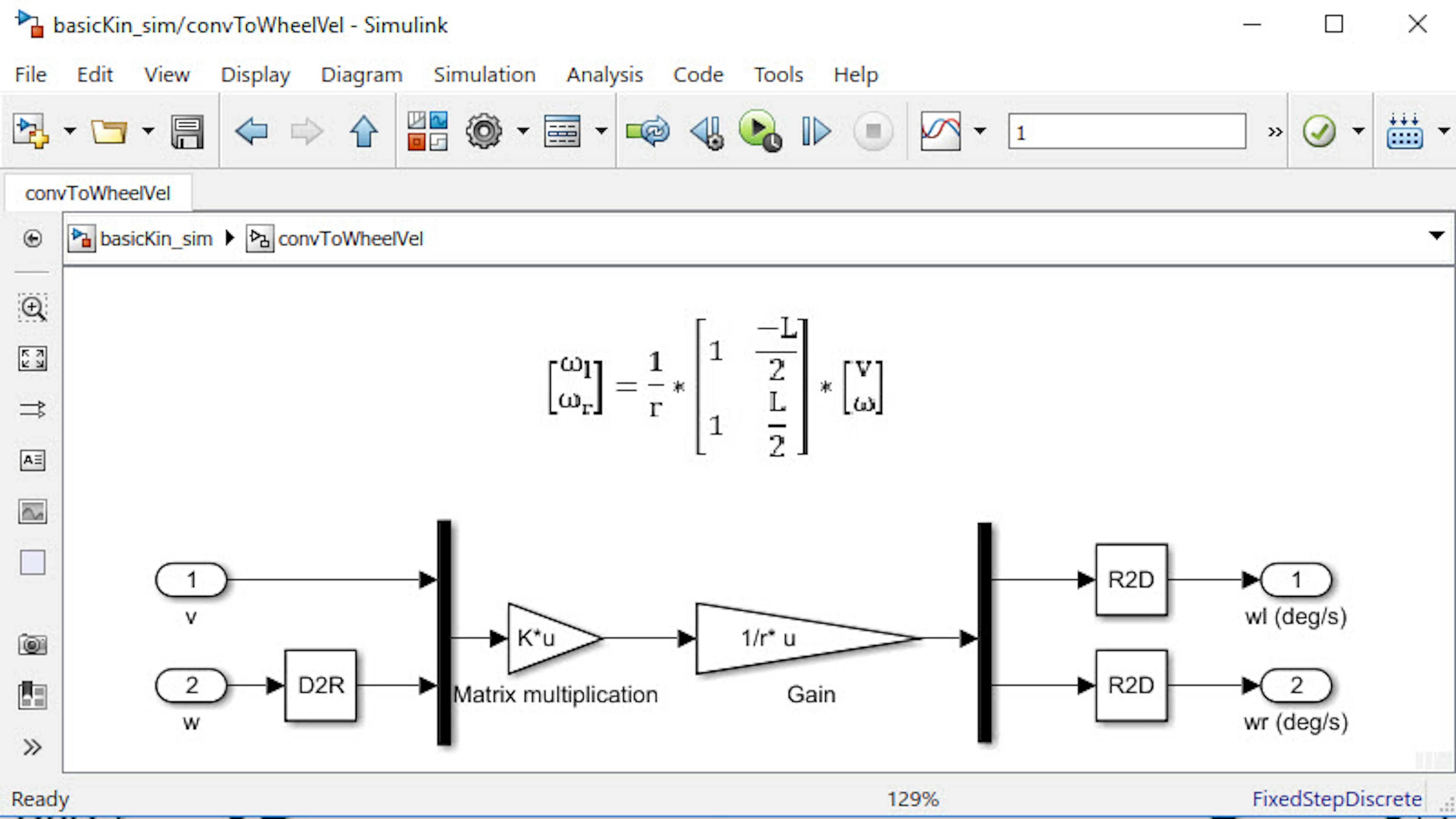
Here you can see the inports (v and ω) on the left side and the outports (ωl(deg/s) and ωr(deg/s)) on the right. The D2R block adjacent to the inport w is converting degrees to radians, while the R2D blocks are doing the inverse operation before sending the resulting data to the outports. The thick black lines are Mux and Demux blocks; they allow us to arrange the data into vectors and separate them back to scalars as needed. This allows us to perform a matrix multiplication with the first triangular Gain block (Ku) on the vector and the second Gain block will multiply the components of the resulting vector with 1/r.
This subsystem calculates ωl and ωr for a given desired velocity and rate of rotation. The equations implemented in this subsystem are displayed within the model for reference. This is a feature in Simulink that allows you to include documentation within the models themselves, which makes it easier to share your work with others.
Let's navigate back to the top-level model by clicking basicKin_sim as shown below.
As an example, try v = 10 cm/s and ω = 0 deg/s and click the Run icon as shown below. Simulink will then perform the computation and update the display once every 0.01 seconds as mentioned by sample time TS . On the display, you should see results consistent with the values calculated earlier, in this case: ωl=ωr=127.3deg/s
Try once more with v = 0 cm/s and w = 18 deg/sec and Run the model again. Results are consistent again and in this case:
$\omega _{l}=-17.6\frac{deg}{s}; \omega _{r}=17.6\frac{deg}{s}$
SIMULATING THE ROVER'S MOTION
In the previous section, Simulink was used to implement basic kinematic equations of the rover, but the model did not consider the location of the rover in real-world coordinates. The location (x, y) and heading (θ) of the rover in an X-Y coordinate system can be described using the following equations:
$\theta \left( t \right) = \int _{0}^{t} \omega \left( t \right) dt~~ x \left( t \right) = \int _{0}^{t}v \left( t \right) \cdot cos\theta \left( t \right) dt~~~~~ y \left( t \right) = \int _{0}^{t}v \left( t \right) \cdot sin \theta \left( t \right) dt$
Let's see how to use Simulink to implement these equations and simulate the rover's movement over time. Start by opening the kinEq_sim model from MATLAB:
>> kinEq_simIn this model, you see that instead of simple constant inputs that were there in the previous model, there are now Signal builder blocks labeled $v (cm/s)$ and $\omega (deg/s)$. These provide signals changing over time to the convToWheelVel subsystem. Instead of simply displaying the results, they will be passed on as inputs to the Rover Simulation subsystem, which mathematically models the rover's behavior and creates a visual simulation of the rover moving around a 100 cm x 100 cm "arena."
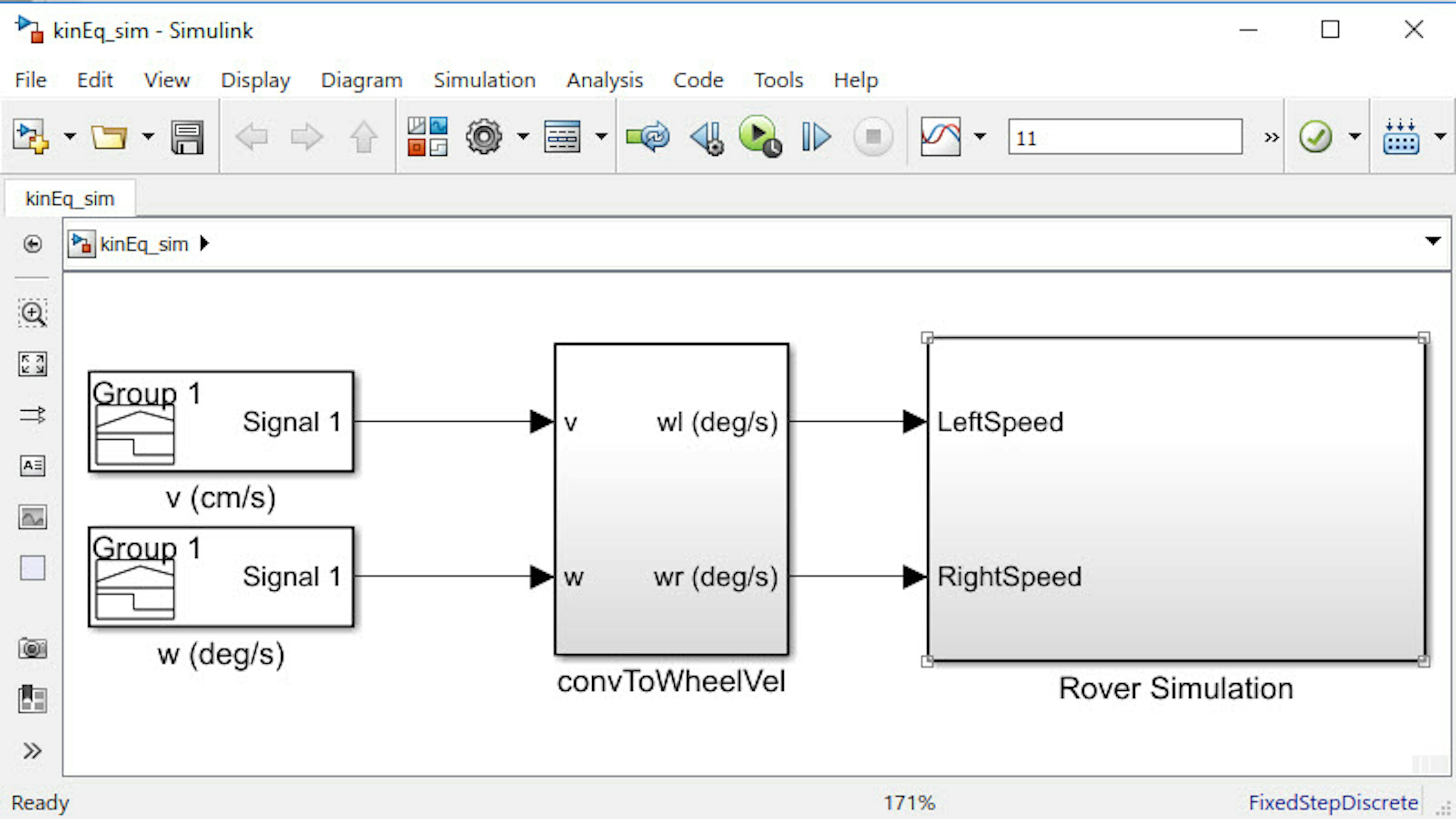
Note: the convToWheelVel subsystem is the same subsystem from the previous model.
Double-click on the v (cm/s) block to see what the signal looks like.
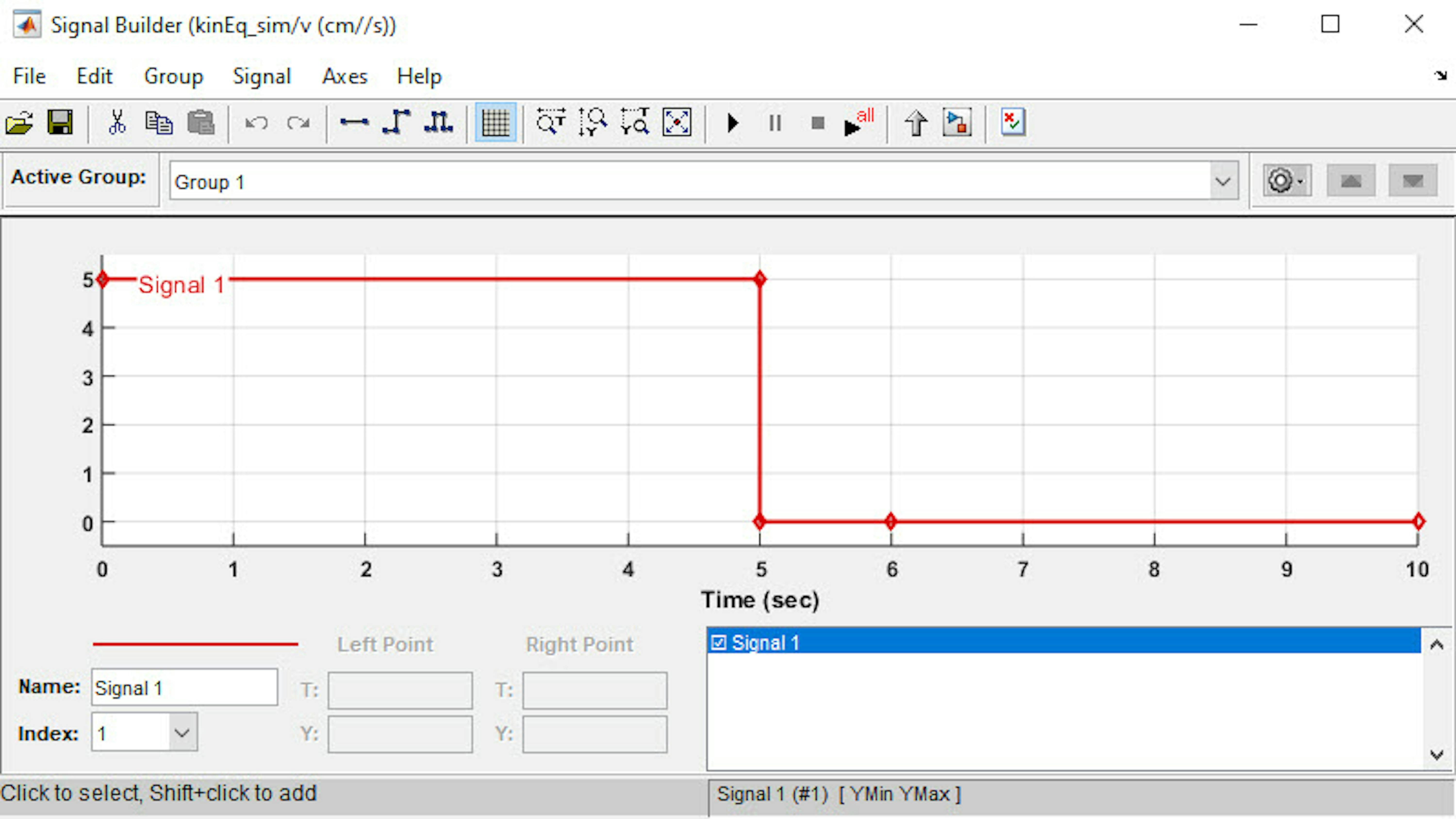
The signal looks like a step that has a magnitude of 5 cm/s for first five seconds and then drops down to 0 cm/s.
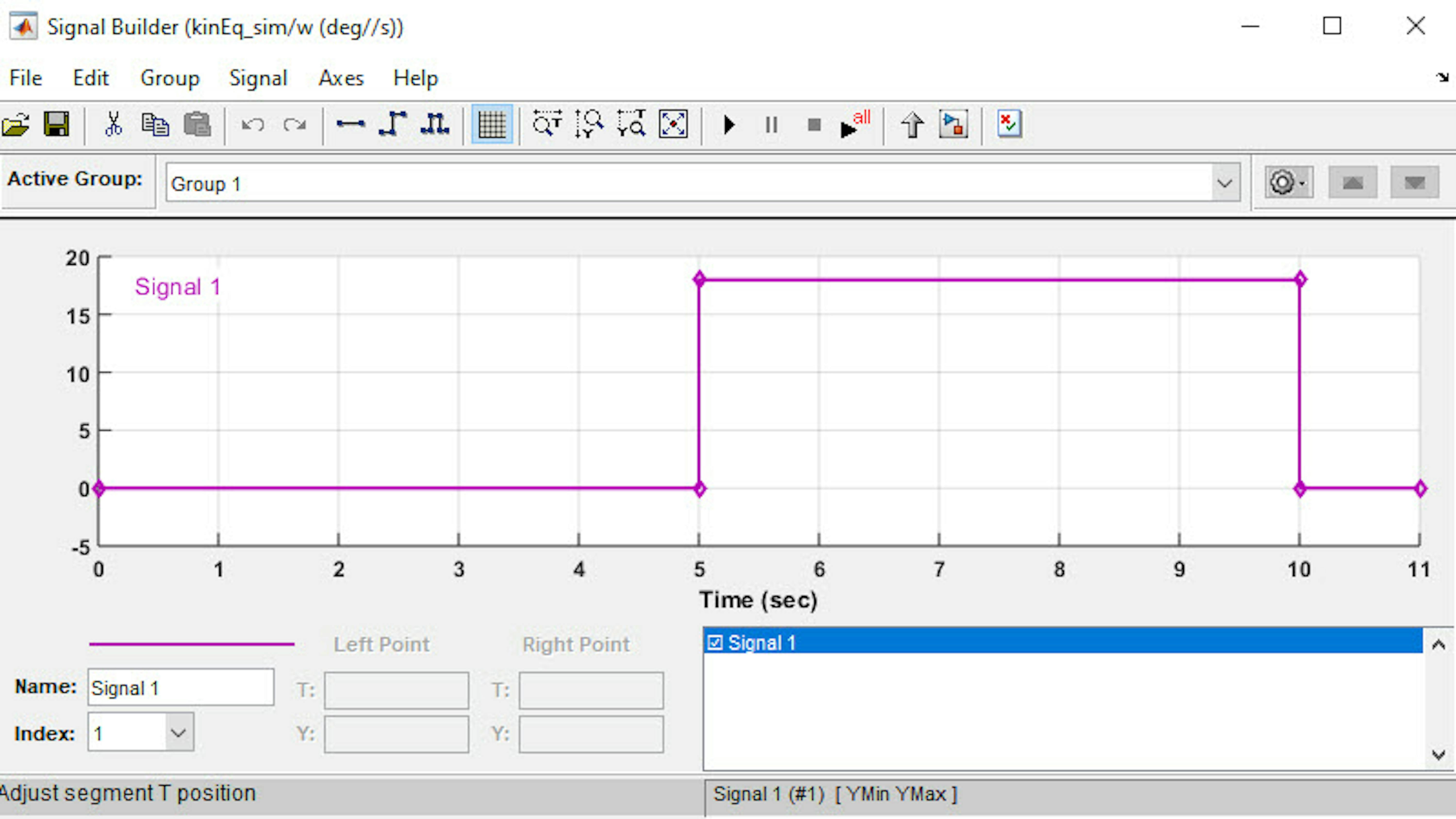
The signal for w (deg/s) is a rectangular signal that has a magnitude of 18 deg/s between 5 and 10 seconds and zero at all other times.
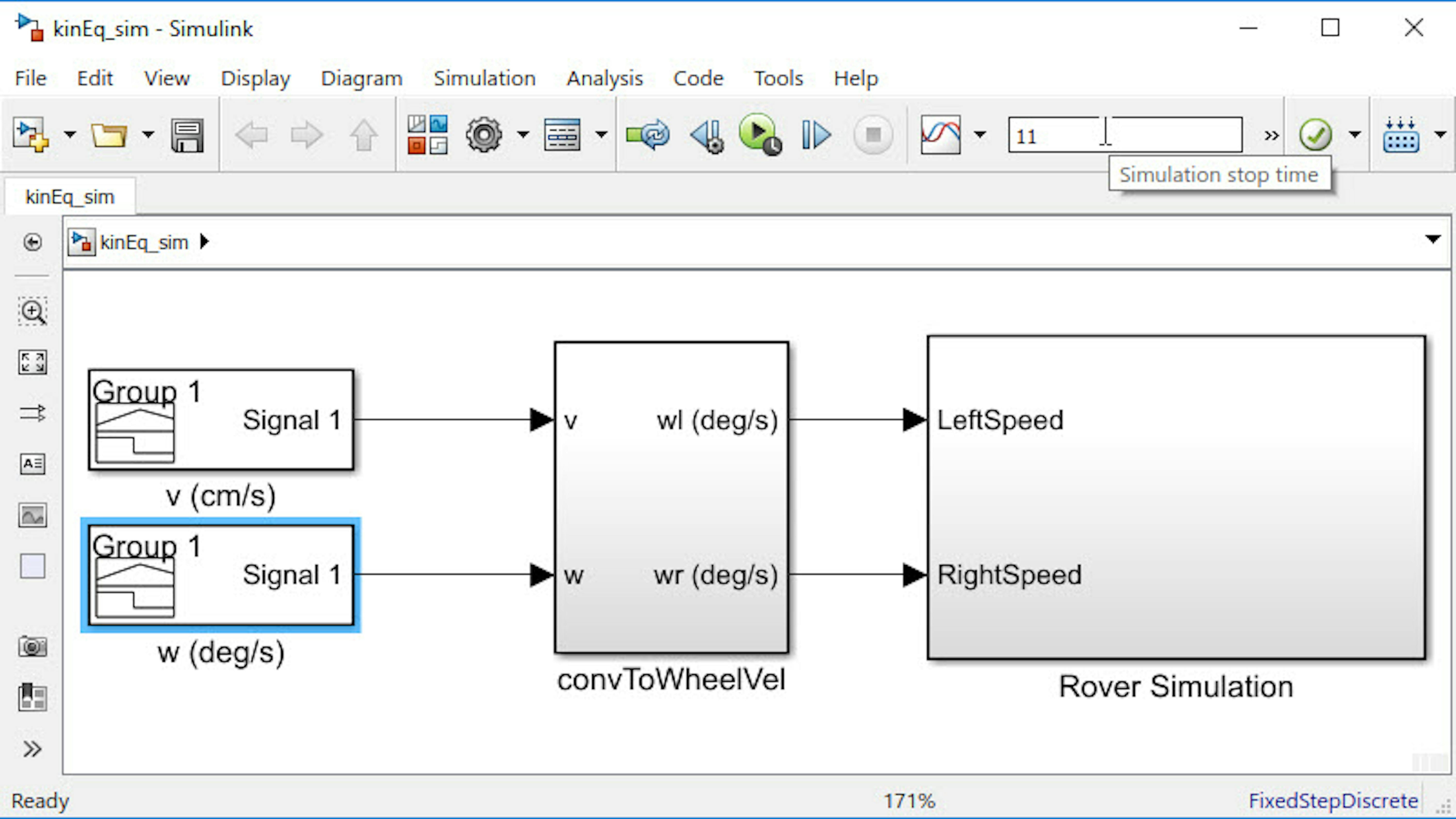
Since the input signals are both zero after 10 seconds, the simulation stop time is set to 11 seconds as shown below.
Open the Rover Simulation subsystem. There are two inports to bring in the angular speed of each wheel and there are three subsystems here: the Encoder simulation, the Vehicle kinematics, and the Robot path plotter models.
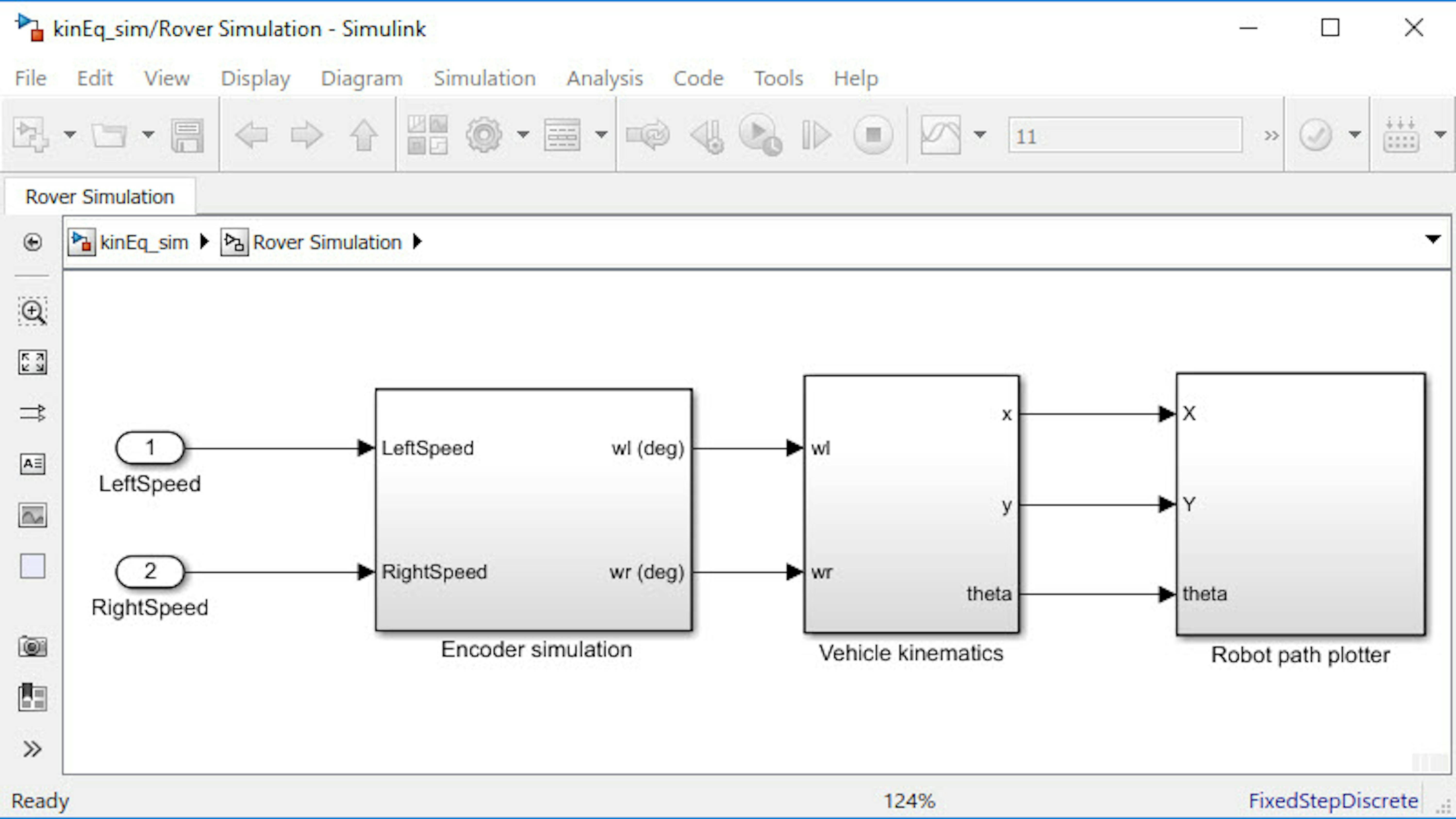
The Encoder simulation subsystem converts the desired wheel rotational speeds from deg/s to degrees rotated by the wheel, to mimic the encoder on your rover. To learn more about the actual encoder used and its behavior, refer to the section 2.3.2.3 Reading encoder count in "2.3 Simulink Getting Started".
The Vehicle kinematics subsystem implements the equations for θ(t), x(t), and y(t) introduced earlier. Open this subsystem . At this point, you know enough about Simulink to find more information about each one of the blocks. Spend as much time as you need to understand how the equations translate into the following block diagrams. Essentially, you will see that the outports are the result of integration operations, and the outports are the orientation of the rover and its x and y coordinates.
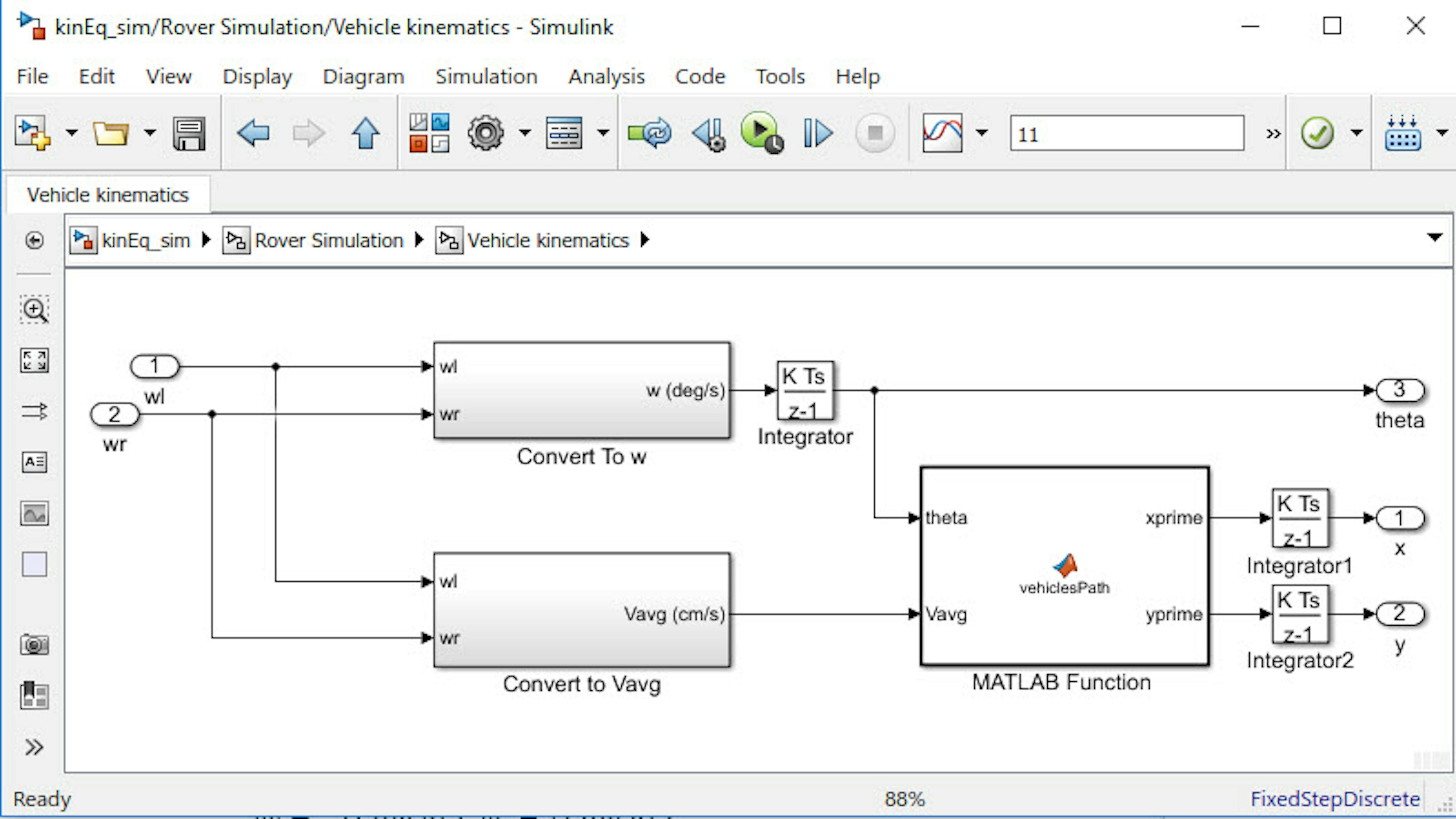
Explore the vehiclesPath MATLAB Function block to see how the equations are implemented here. A MATLAB function block allows you to integrate MATLAB code within Simulink models.
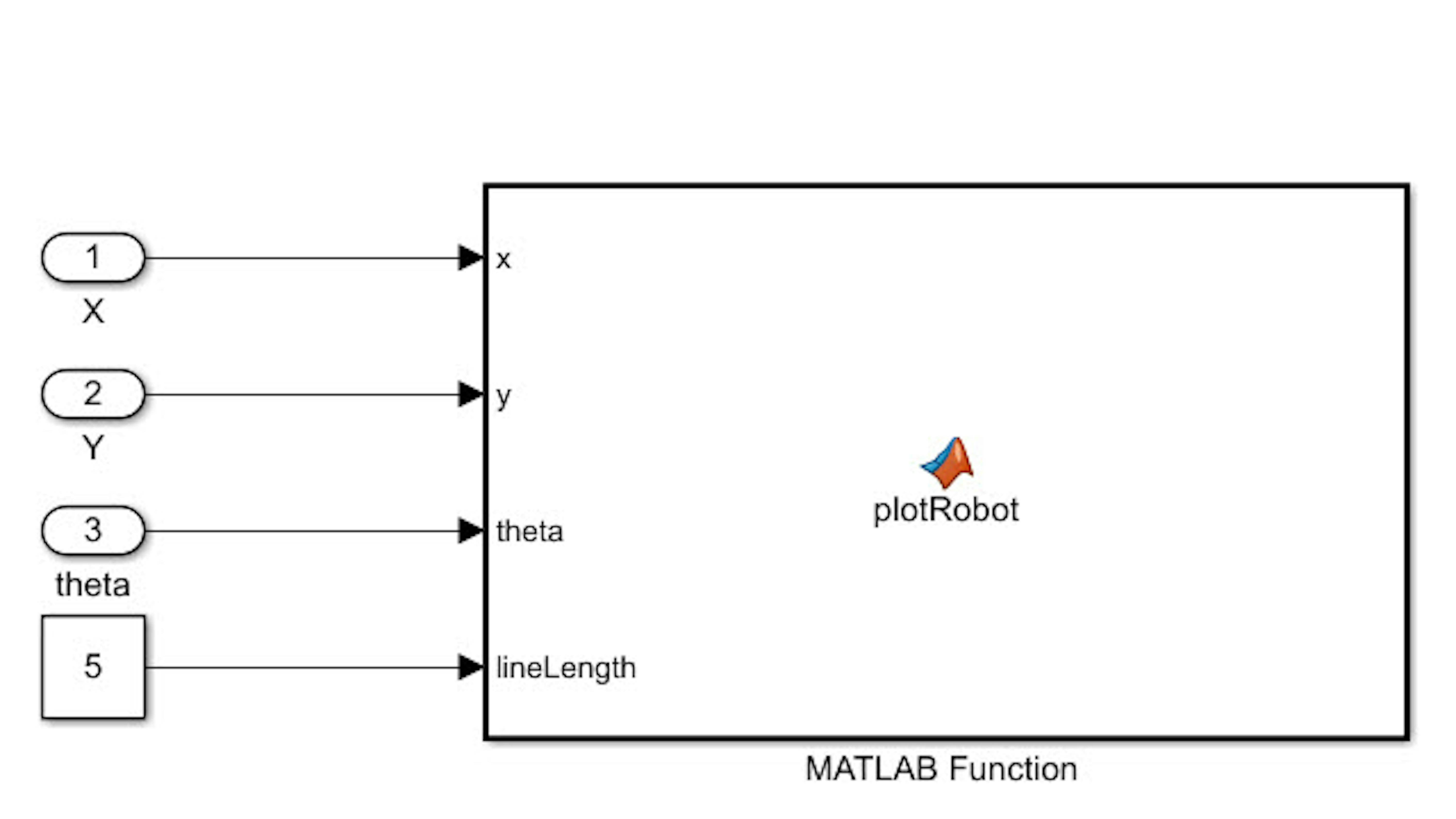
Navigate back to the Rover Simulation subsystem and open Robot path plotter subsystem.
You will see how there is a constant block besides the inports that is sending the value 5 to the MATLAB Function block. This is used to draw the robot's trajectory. Open the plotRobot MATLAB Function block to see how to visualize the robot's path x, y, and θ change with time.
Once you are familiar with how the model works, click Run.
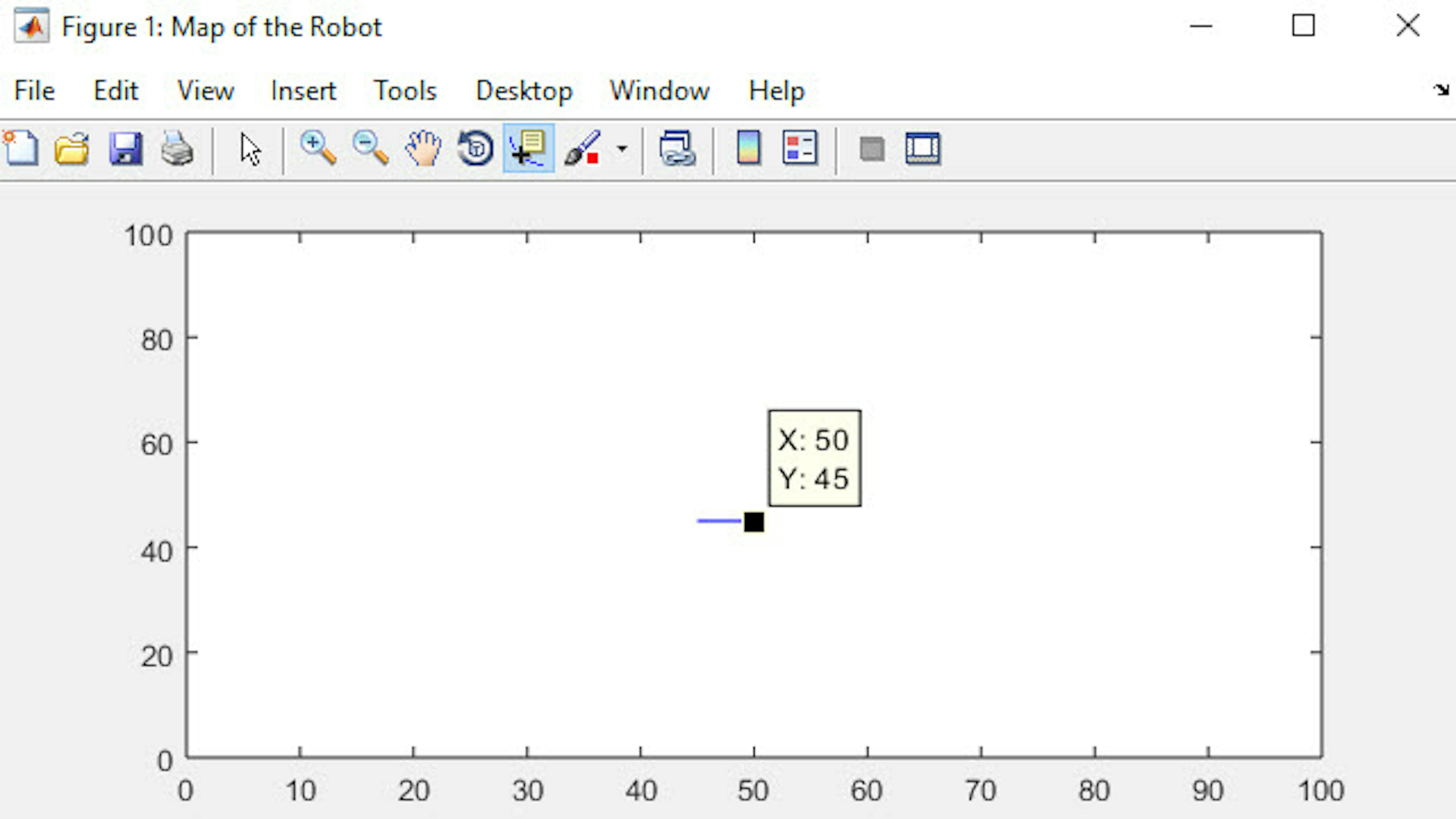
You will see the rover move around the 100 cm x 100 cm arena for 11 seconds. The simulation is based on a starting position of StartX = 50 cm , StartY = 20 cm and StartTheta = 90 deg. These variables were defined earlier in the Workspace through model callback PostLoadFcn just as you saw in the previous model. Overall, the rover moved 25 cm in the y direction and then turned 90 degrees based on the Signal Builder inputs.
DRIVING THE ROVER USING OPEN-LOOP CONTROL
Once you have tried out the simulation, it is time to make the rover do the same maneuver in the real world. We have prepared a Simulink model for you to quickly see how this could work. Open the roverOpenloop_hw model from MATLAB:
>> roverOpenloop_hwThis model resembles the one in the previous section, except that instead of sending wheel velocities to a mathematical model of the rover, the outputs are going to be sent to the motors mounted on the real rover.
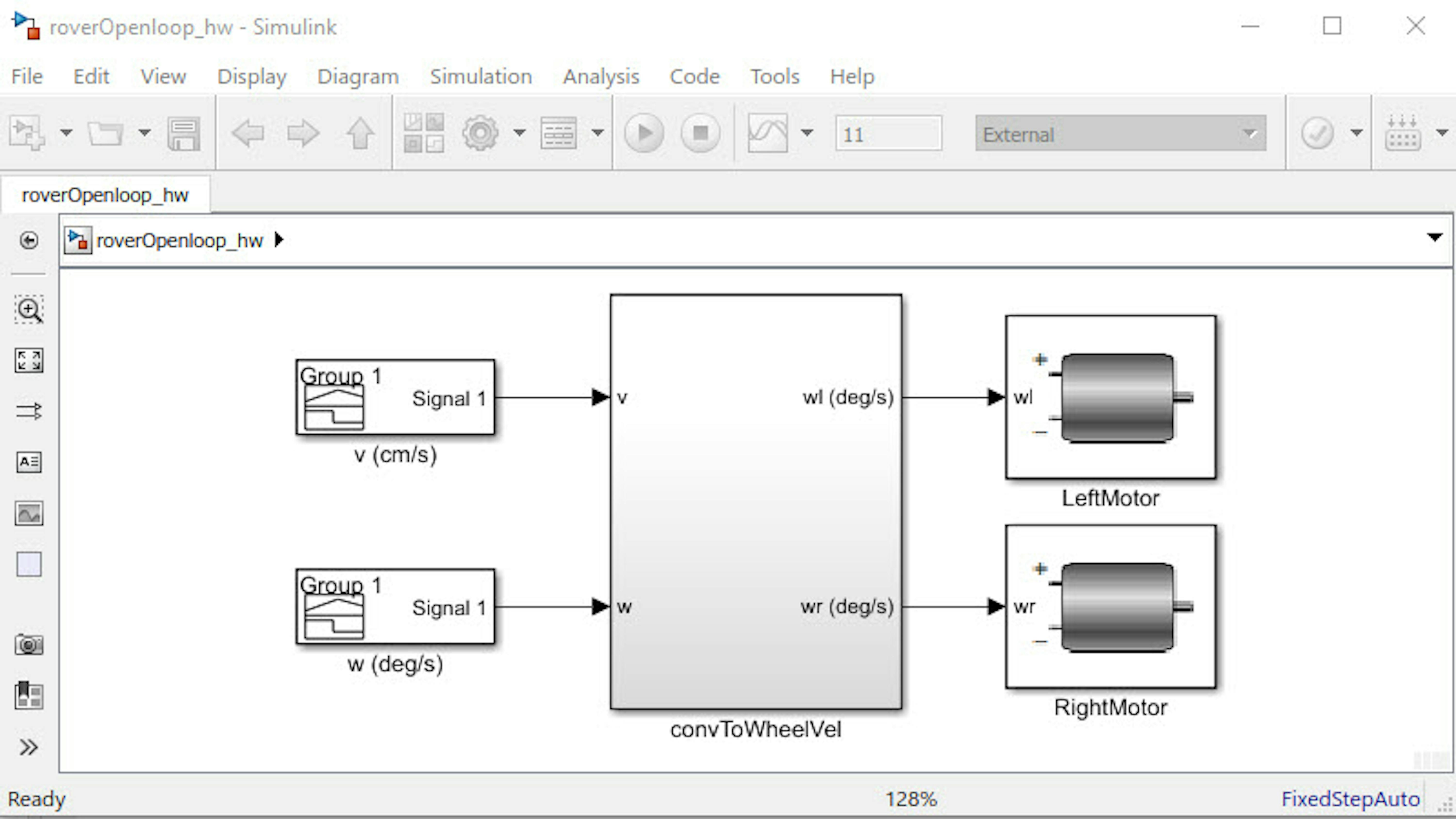
The input signals and the convToWheelVel subsystem are the same as the previous model, but the rotational speeds are sent directly to the actual motors that are presented as blocks inside the model.
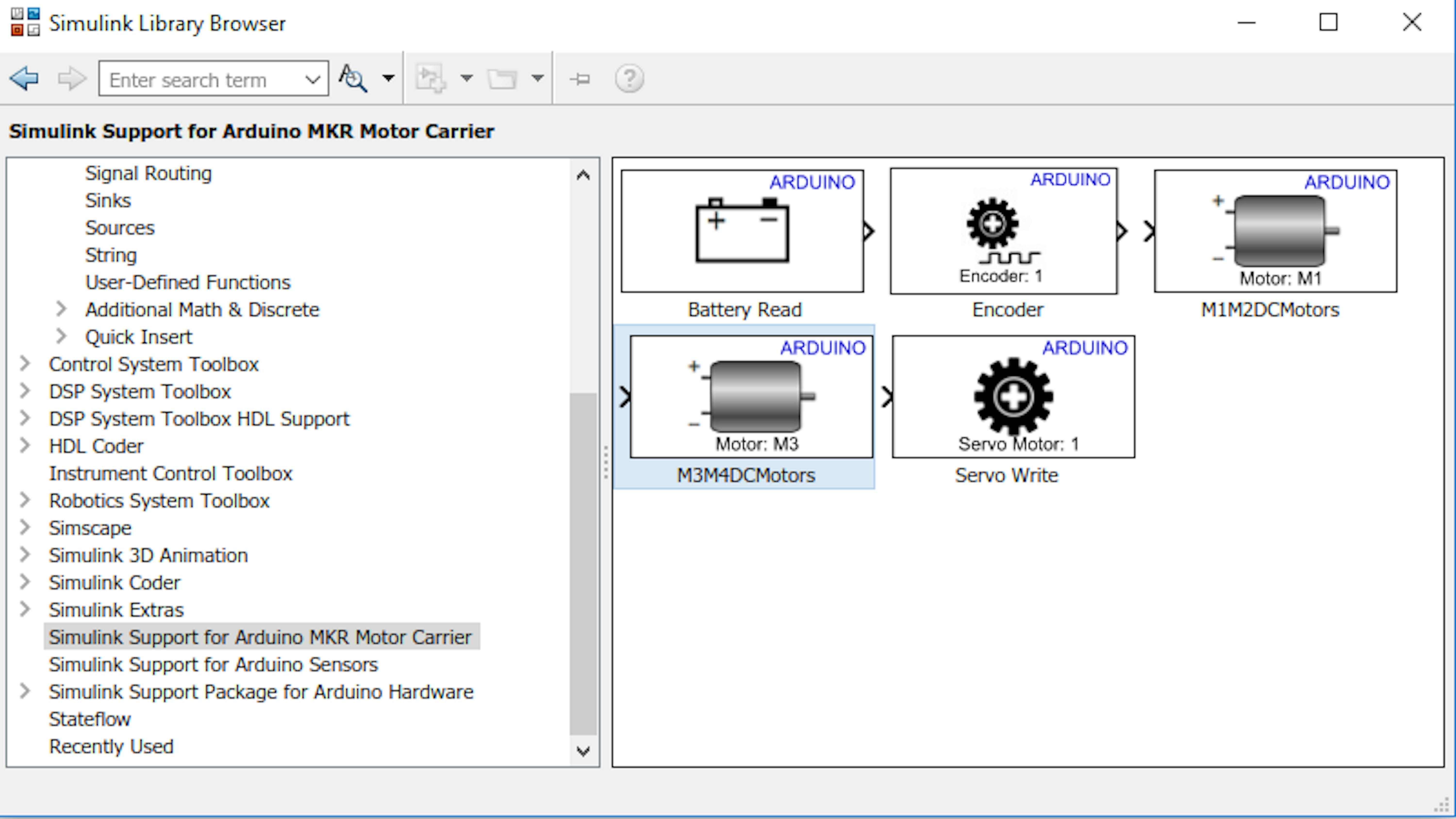
The LeftMotor and RightMotor blocks come from the library Simulink Support for Arduino MKR Motor Carrier as shown below.
As discussed in section 2.2.3 Characterizing a DC Gear Motor in "2.2 MATLAB Getting Started", the input to the Motor blocks should be a PWM signal, not a commanded rotational speed. So, inside the LeftMotor and RightMotor subsystems, the commanded rotational speeds are converted to PWM using new motor characterization data. The reason behind the need for new characterization data is the motor characterization in section 2.2.3 in "2.2 MATLAB Getting Started" was done when the rover's wheels were spinning freely in the air. The new motor characterization was performed with the rover moving on the floor and the battery having full charger. The provided data (Data.xlsx) for the rover shows relationship between PWM value and commanded motor speed. This is represented by the Lookup table block within the LeftMotor and RightMotor subsystems.
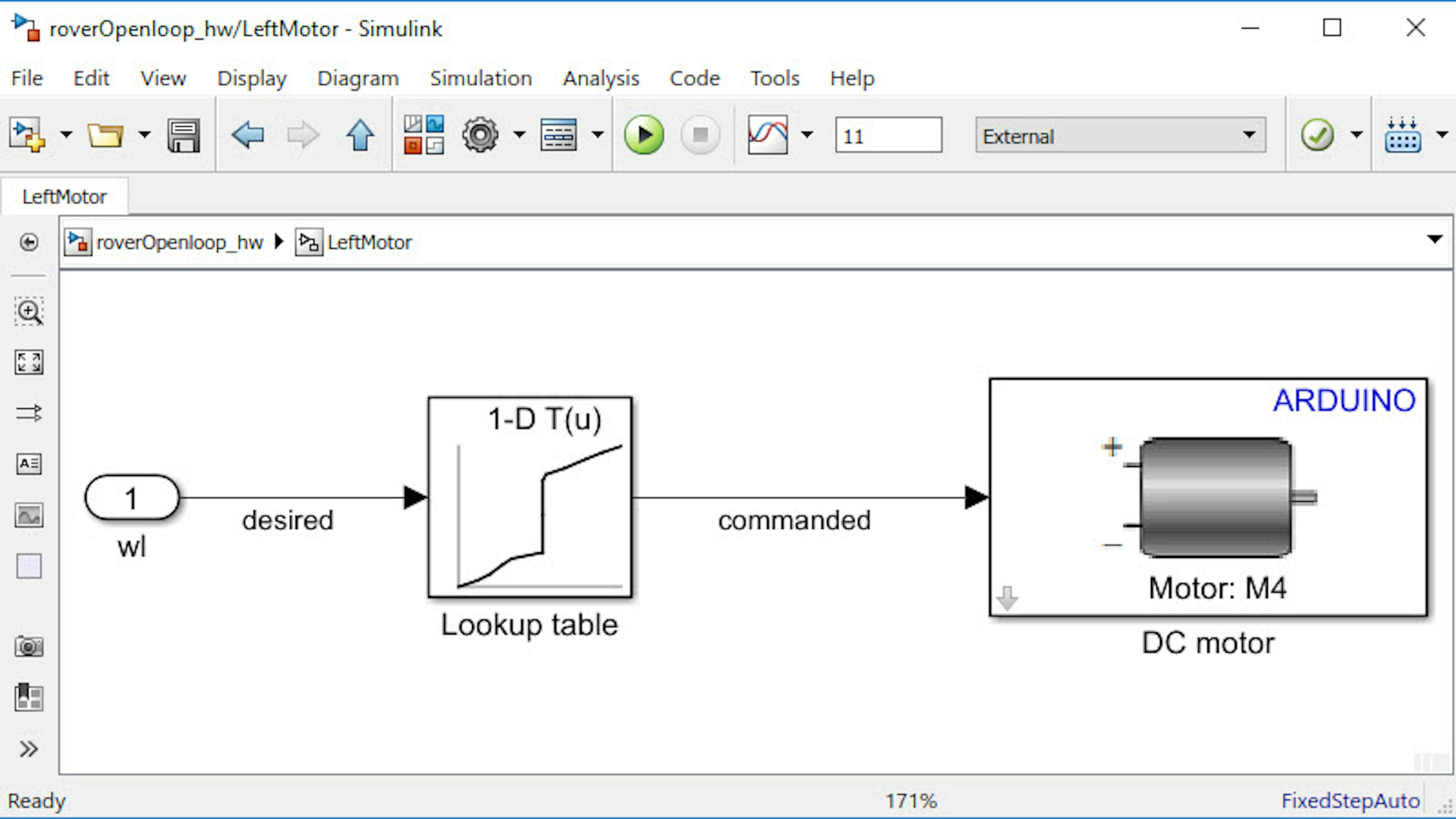
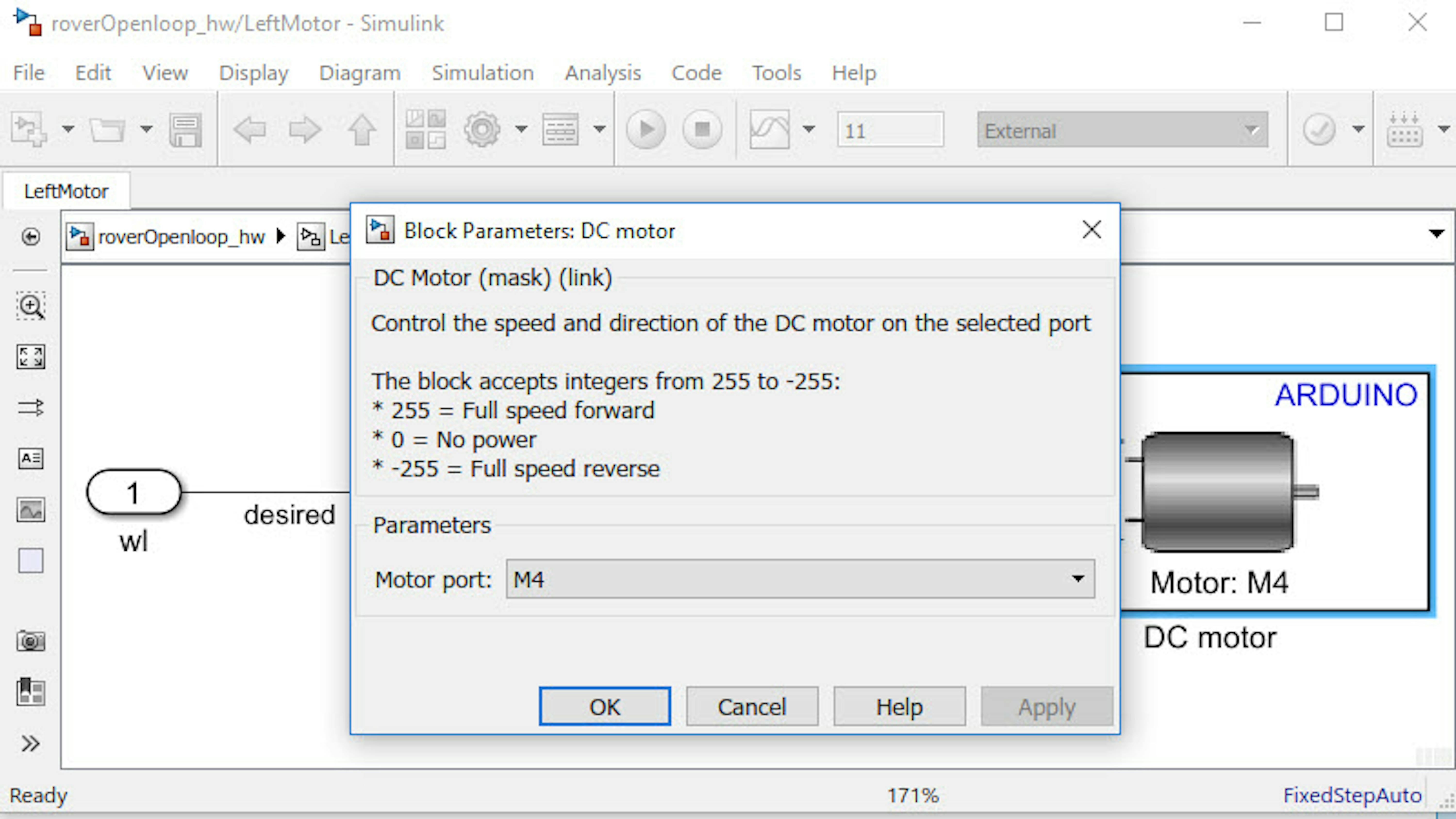
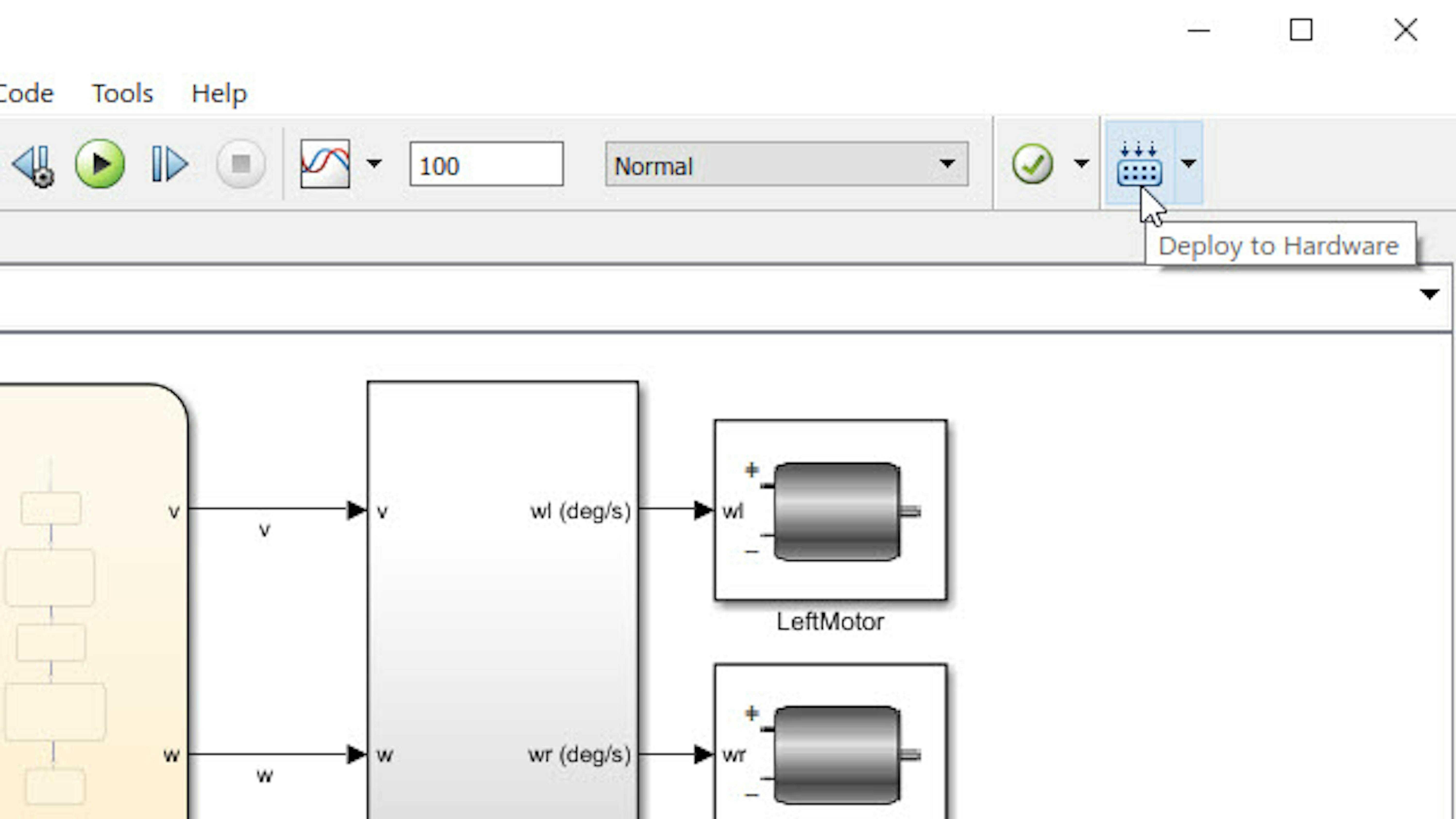
Check the port numbers specified by the DC motor blocks in the LeftMotor and RightMotor subsystems to ensure that the connections for the right and left motors of your rover match the ones specified in these blocks. The image below shows the DC motor block inside the RightMotor subsystem.
Important: Connect your rover to the computer using the USB cable without powering on the battery.
Press the Deploy to Hardware button in the model window toolstrip. This will generate the code equivalent of your model and upload it to the Arduino MKR1000, which will ensure that the rover can run the code on the board even when it is detached from the computer.

Disconnect the USB cable from the rover and place the rover on the floor or some other surface where it has enough space to move around. The rover is fragile, and it could get damaged if it fell from your desk.
Power on the rover (using the battery) and measure the distance it covers on the floor. Your goal is to check whether the real experimental conditions replicate what you simulated in the model earlier.
Recall that in simulation the rover moved 25 cm in the y-direction and then turned 90 degrees. Did the real-world rover do the same?
You're likely to see that it did not. In general, it's very difficult to accurately control your system using open-loop control unless you have a very accurate model of your motor behavior and operating environment. In our case, the motor characterization was not rigorous and a simple relationship for PWM versus motor speed was used. That said, even if the characterization were rigorous there would be issues if you want to operate the rover on a surface different than the surface used for motor characterization, or if the battery is not operating at the same voltage.
NEED FOR CLOSED-LOOP CONTROL
In the next exercise, you will see how closed-loop control will help address the limitations observed with open-loop control and enable much more accurate control of the rover position.
REVIEW/SUMMARY
-
We saw how to use kinematic equations and inverse kinematics to simulate the rover movement.
-
We saw how to translate that understanding to control the rover in the real world.
-
We saw that the mathematical modeling needs to be tweaked to better accommodate real-life conditions.
FILES
-
basicKin_sim.slx
-
kinEq_sim.slx
-
roverOpenloop_hw.slx
-
roverMotors_hw.slx
-
Data.xlsx
LEARN BY DOING
Try updating input signals in the Signal Builder block using various combinations of v and w. Can you make the rover move in a circle, or follow a specified sequence of movement (for example, forward 20 cm in y-direction, turn 90 degrees, forward 20 cm in x-direction)?
EXERCISE 3
5.3 Closed-loop control of Rover position
In this exercise, Simulink will be used to implement a PI controller that controls the distance moved by the rover. You will see how to read the encoder data from the rover's wheels and use this data as feedback to your controller. You will also see how to tune PI values of the controller to optimize performance.
In this exercise, you will learn to:
- Understand basics of a PI controller design and, by extension, PID controllers.
- Read encoder data.
- Tune parameters of a controller in Simulink.
- Implement a controller on the rover.
BASICS OF A PID CONTROLLER
A proportional integral-derivative-controller (PID) is a control-loop feedback mechanism used in systems requiring continuously modulated control. PID controllers operate on the error term, the difference between actual and desired behavior, and apply a correction to your system based on the Proportional, Integral, and Derivative terms associated with the error. This has the effect of making corrections for past error (I), present error (P) and future error (D). The correction is denoted by the equation:
$u=Kp\cdot e+Ki\cdot \int _{}^{}e dt+Kd\cdot\frac{de}{dt}$
Where Kp (in Simulink's PID Controller block this is represented by letter P), Ki (I), and Kd (D) are constants coefficients that define the system. This exercise will introduce some concepts associated with PID control in the context of the mobile rover project. Refer to this link for additional information.
CONTROL ROVER POSITION USING A PID CONTROLLER
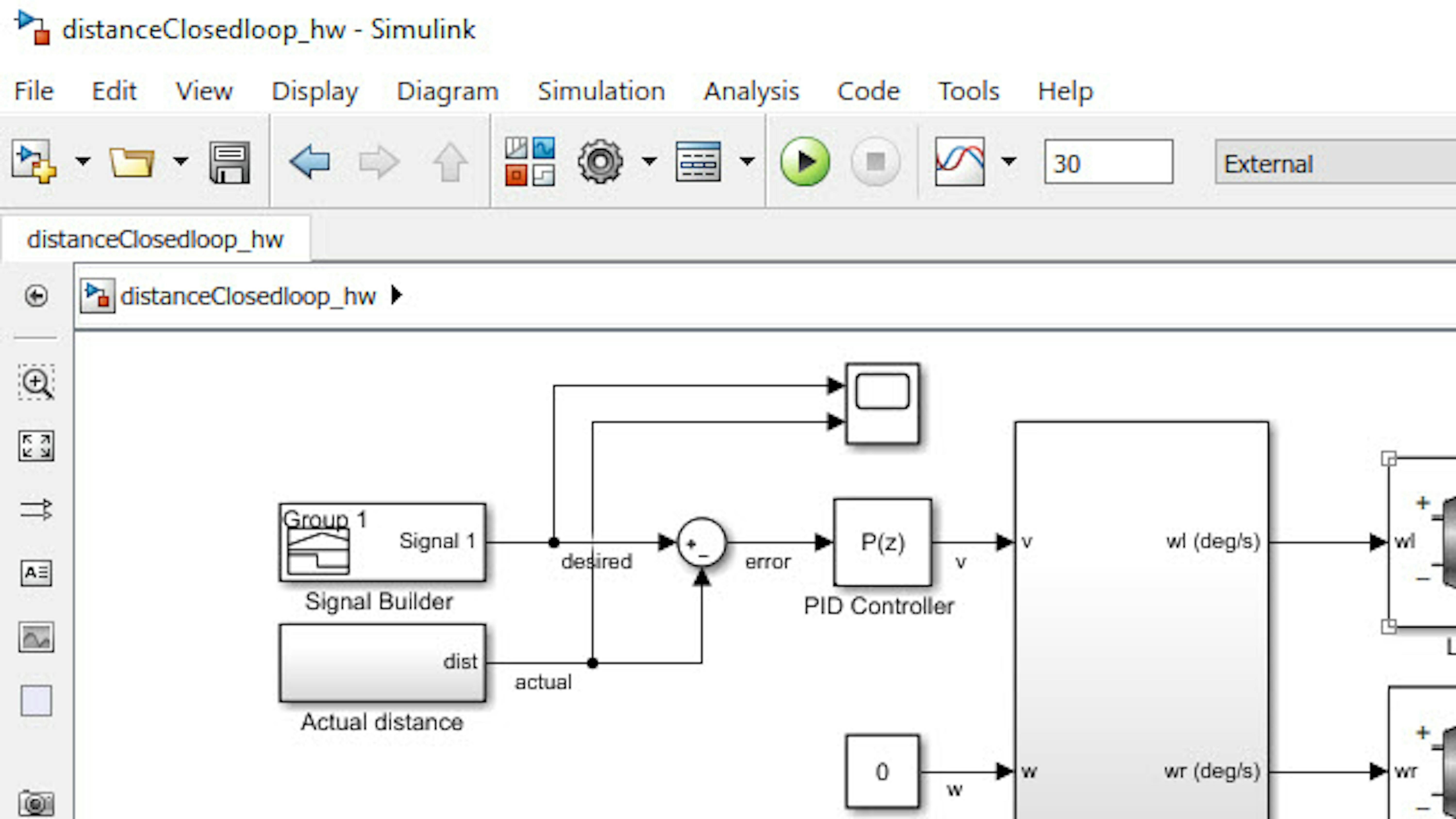
In Exercise 2, the limitations of using open-loop control to control the rover's position were mentioned. Let's see how closed-loop PID control can address these limitations. Start by opening the distanceClosedloop_hw model:
>> distanceClosedloop_hw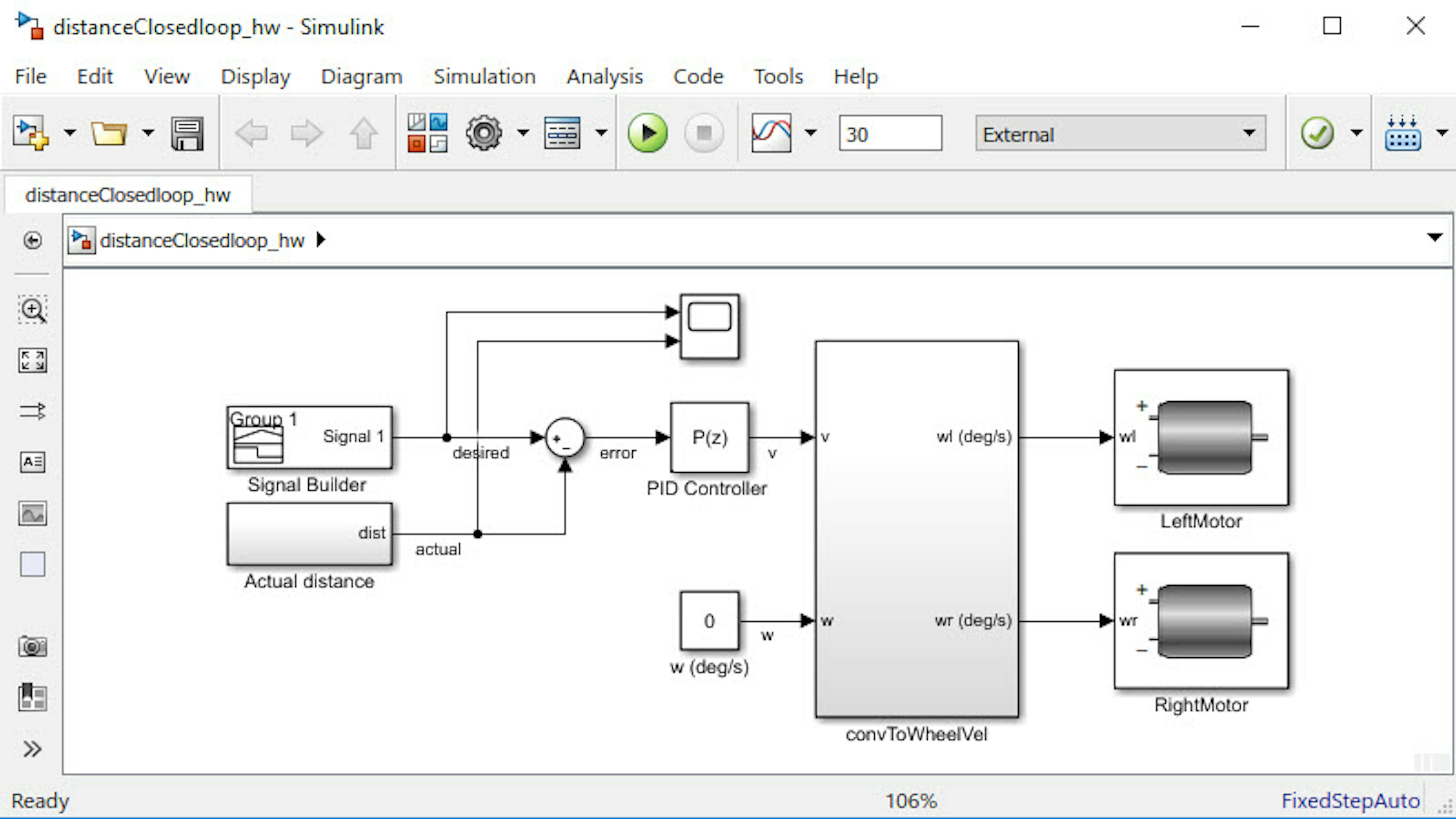
The right side of this model is the same as the roverOpenloop_hw model from the previous exercise. The difference is that the velocity input to the convToWheelVel subsystem is now based on the error term between the rover's actual and desired distance. The challenge will be to determine the actual distance by means of a sensing device on the rover. In this case, the rotary encoders can be used for the same, as you will see later.
To simplify the controller design at the early stages, let's consider the rover moving in a straight line. In this case, the commanded rate of rotation for the rover is zero. In the next section, you will see how to control the rover's angle of rotation.
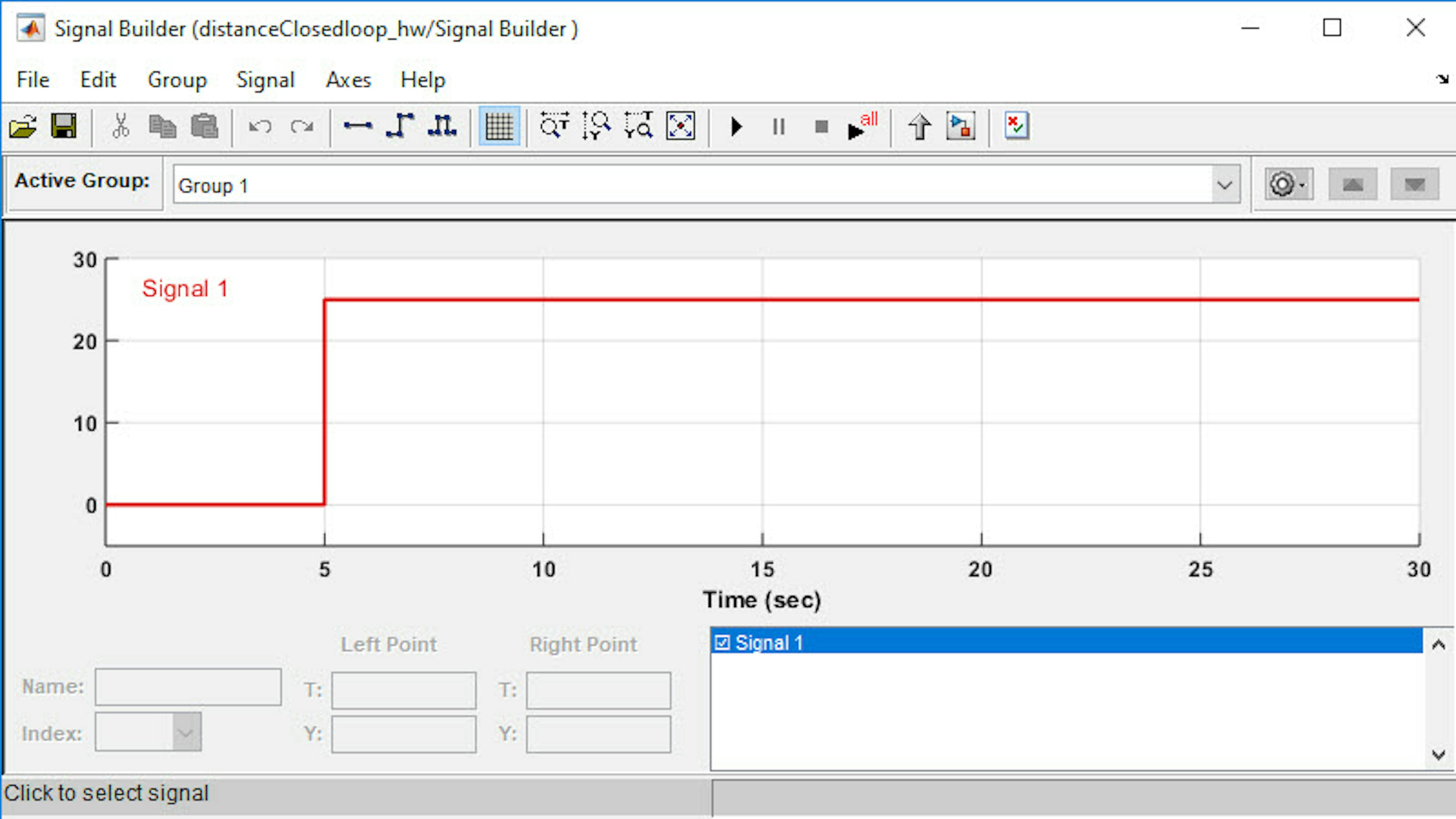
The desired distance is specified using the Signal Builder block. Double-click and open this block. Note how the specified step input of 25 cm occurs at 5 seconds. The following image shows the time diagram for the signal.
As mentioned earlier, the sensor that will determine the distance traveled by the rover is the encoder. Measured distance from the encoder is read into the model in the subsystem labeled Actual distance. Open this subsystem and observe the different blocks that compose it.
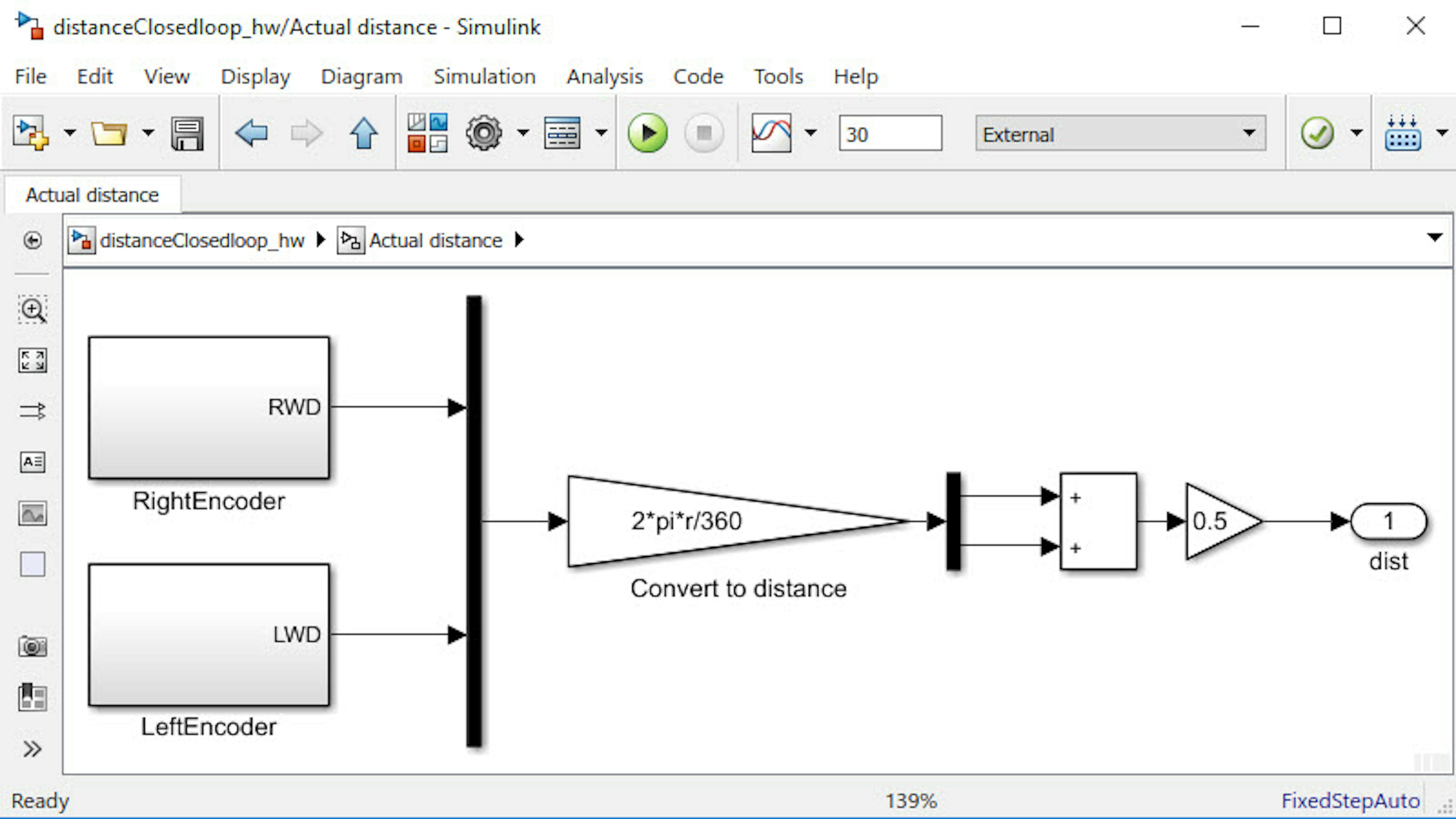
There are two subsystems: RightEncoder and LeftEncoder. The outputs from these subsystems will be arranged into a vector before being multiplied by a constant to convert the encoder readings to distance. The constant is based on the system's characteristics, namely the wheel's radius. The result will be computed into an average and sent to the dist outport.
The RightEncoder and LeftEncoder blocks read count data from the wheel's encoders and convert that to degrees. To convert encoder degrees to the distance moved by the wheels, the following equations are used:
$dr=\frac{ 2\cdot \pi \cdot r \cdot RWD}{360};dl=\frac{2\cdot \pi \cdot r\cdot LWD}{360}$
Here dr and dl denote the distance moved by the right wheel and left wheel respectively and r is the wheel radius.
Navigate back to the top-level distanceClosedloop_hw model and notice how the error is calculated as the difference between desired and actual distance. This is used as the input to the PID Controller.
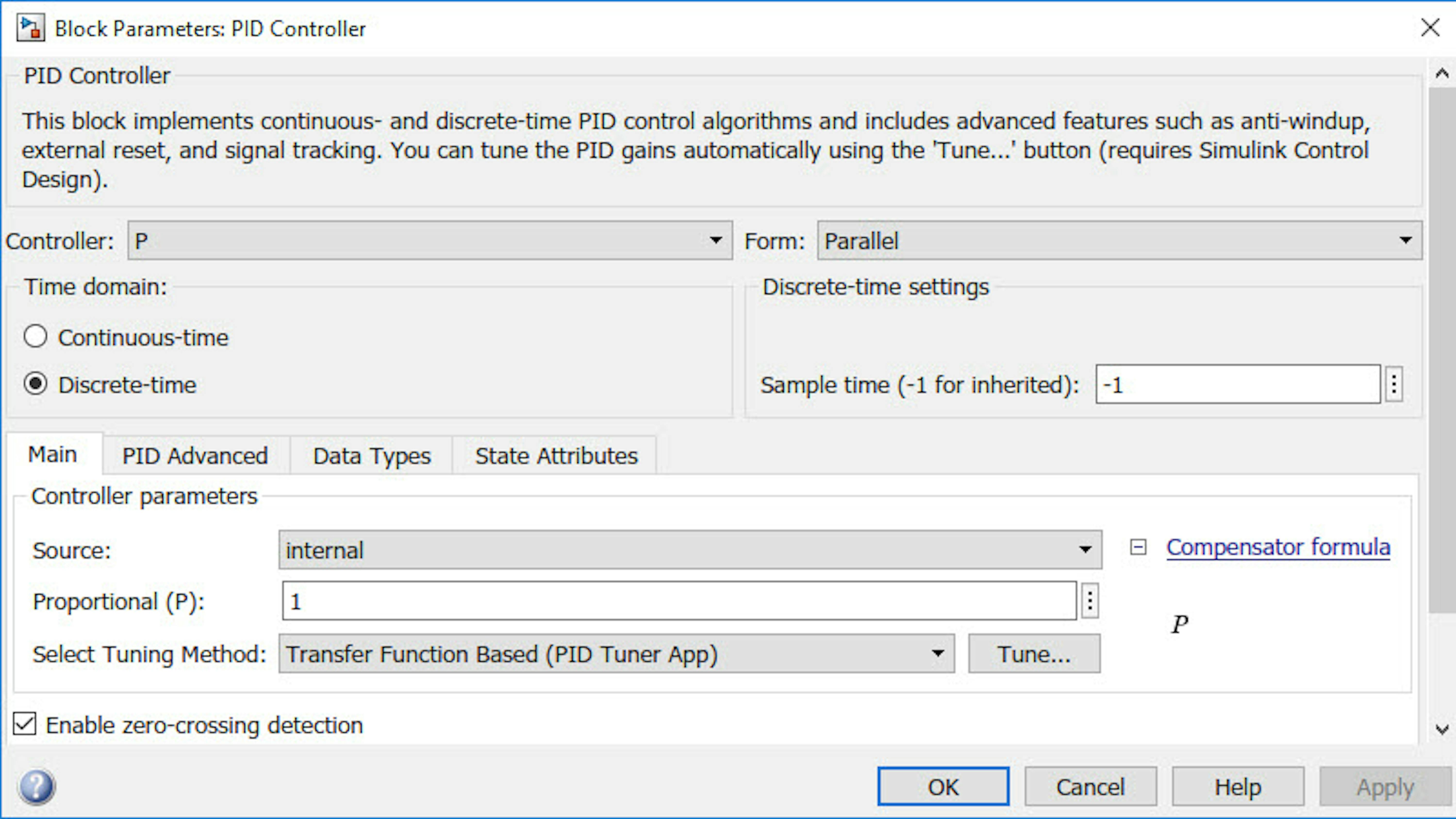
Open the PID Controller block and note that by default a simple P controller is used, since the Integral and Derivative terms (Ki and Kd) are both zero.
You are going to test this on the rover using Simulink's external mode. In external mode, Simulink builds an executable from the model and downloads it to the Arduino. The connection with Simulink is maintained as the executable runs on the hardware, so you can tune parameters and monitor signals of interest using Scope blocks. Refer to 2.3.2.2 Driving a DC motor in "2.3 Simulink Getting Started" for more information about external mode.
Make sure the simulation mode is set to External and simulation stop time is 30 seconds.
For convenience and to help you learn some of the concepts behind PID control, start by putting the rover on top of the target or some other platform that allows its wheels to spin freely. Your rover must be connected to the computer by the USB cable, which means it cannot move far. Turn ON the rover battery as that is where the motors are getting their power from.

Run the Simulink model. After downloading the code to the Arduino, the Scope block will open automatically, which will help visualize desired and actual position as the executable runs.

The result of the scope shows, in this case, the desired distance in yellow and the actual distance in blue. You can see that there is a small discrepancy between them. PID controllers try to compensate for these errors.
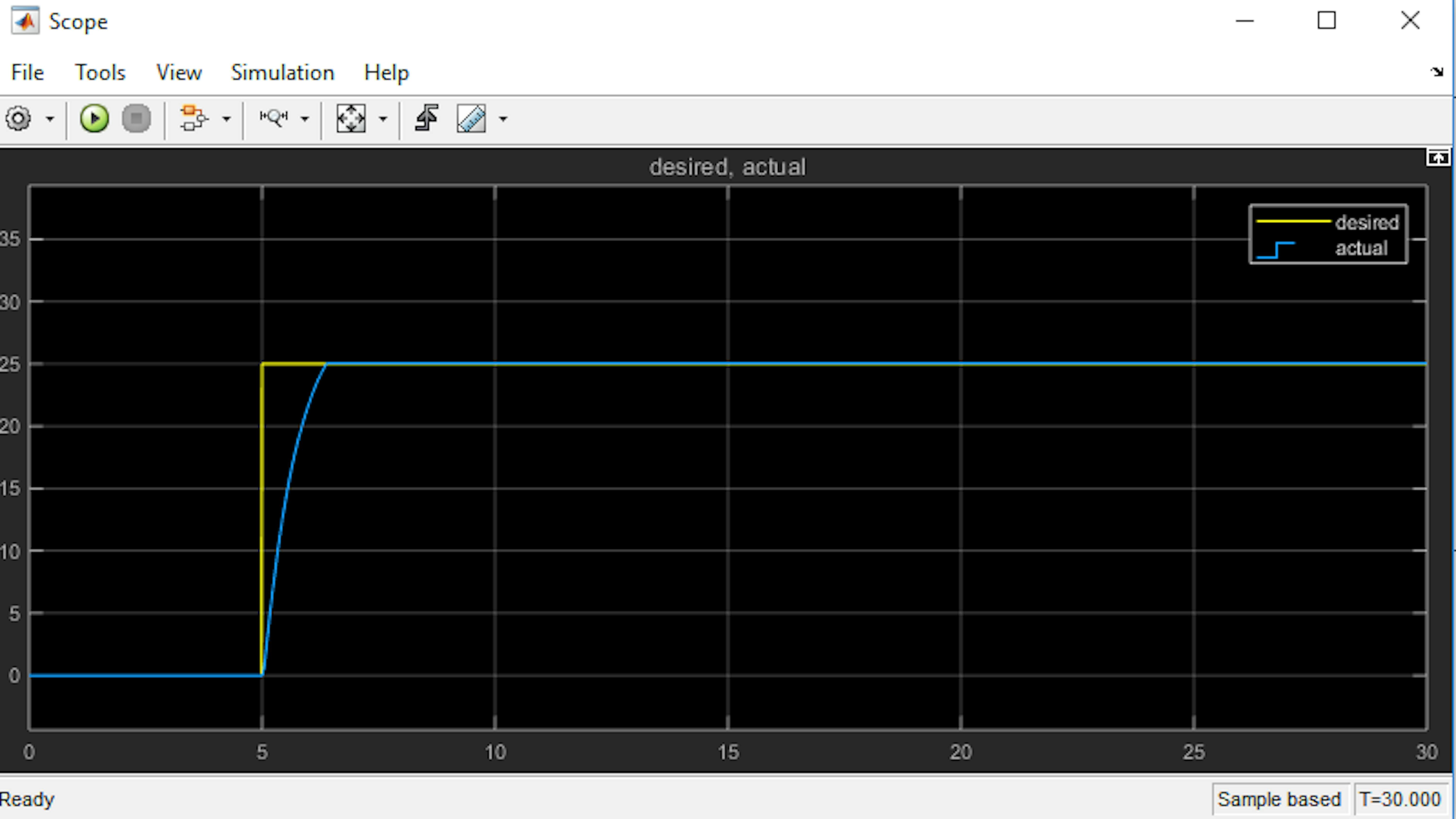
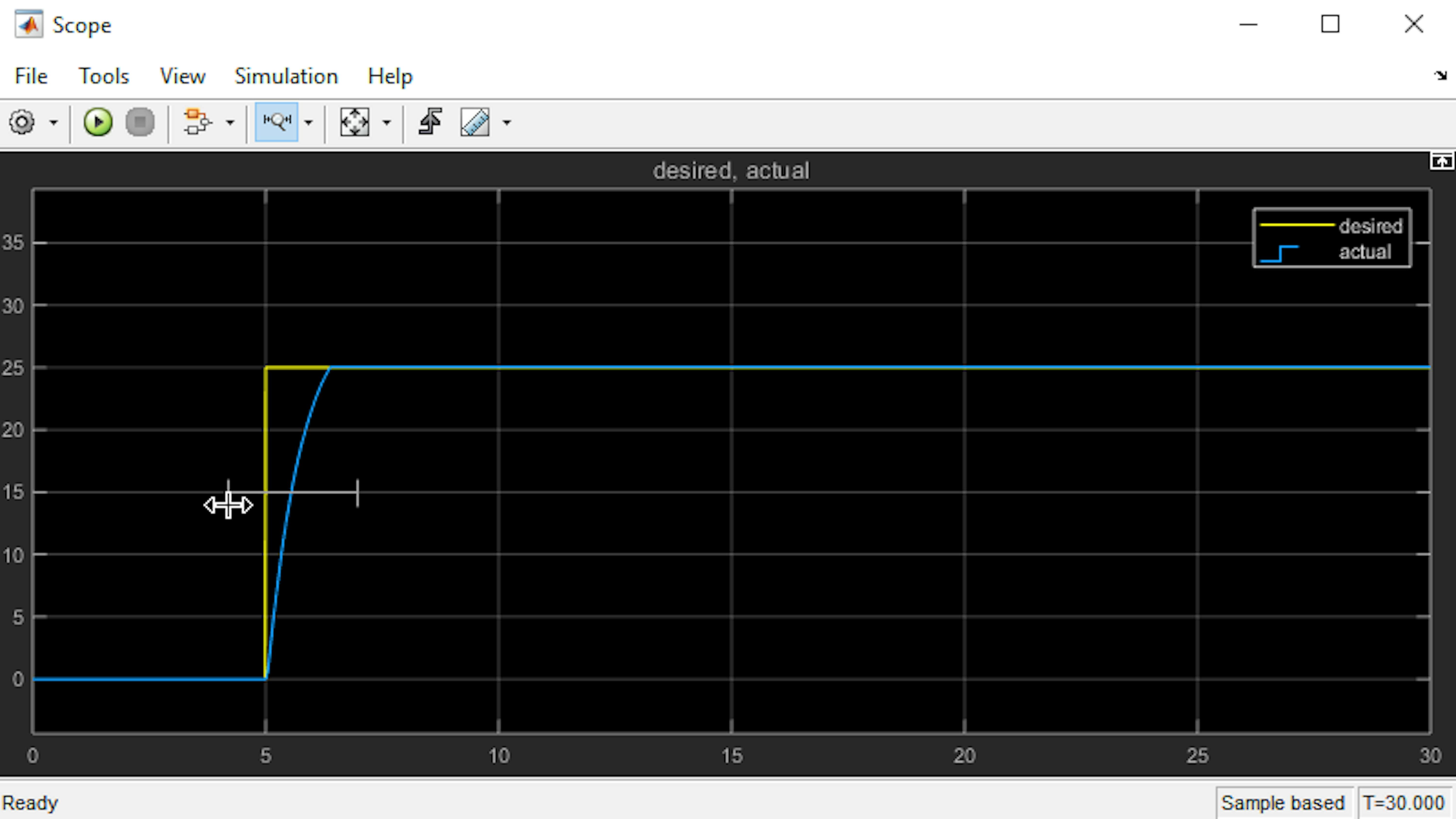
Zoom in on the x-axis to get a closer look at the step response. To do so, click the magnifying glass on the toolbar and select the area you want to zoom in by clicking and dragging on the graph as shown below.
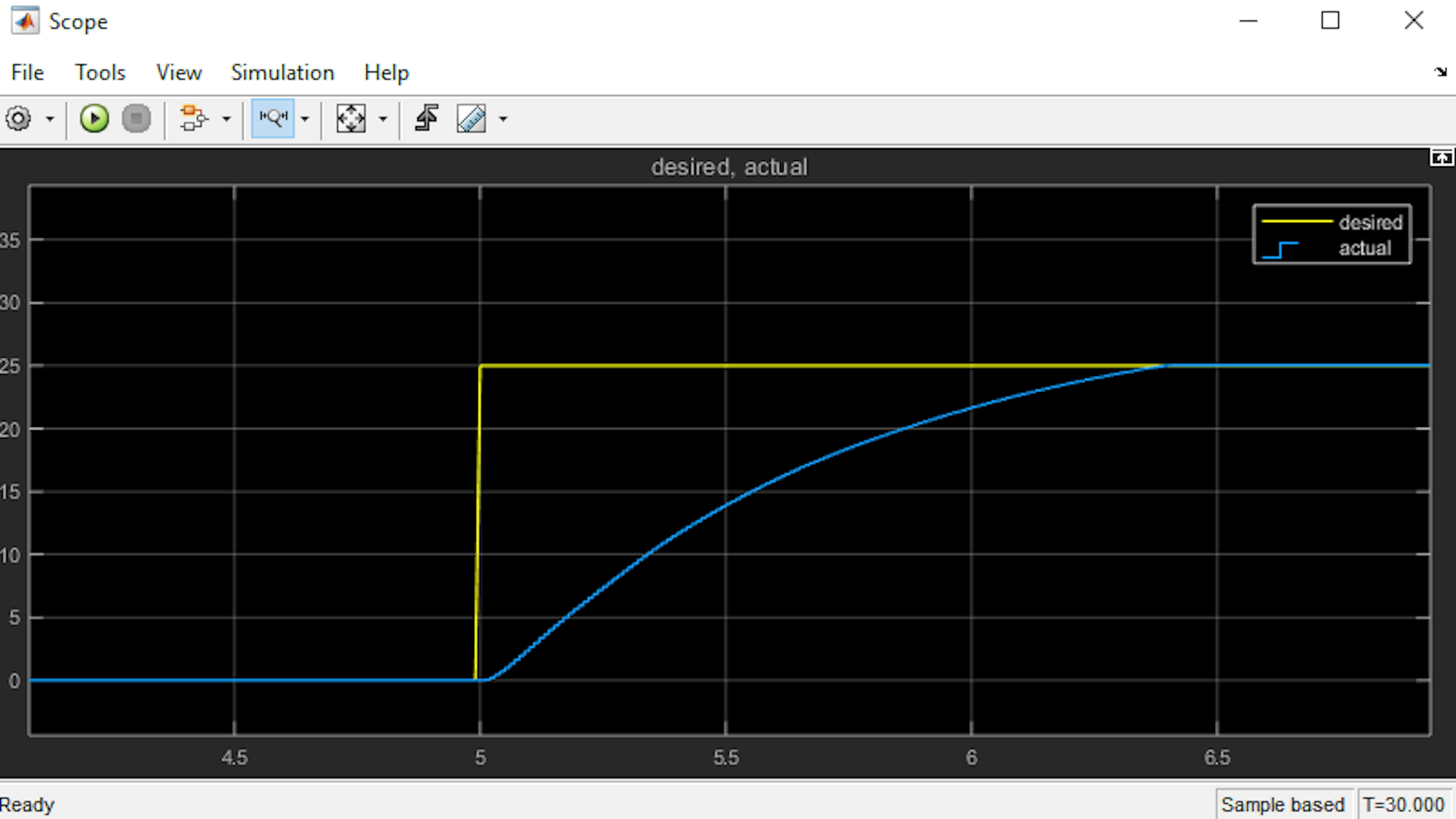
The time it takes to reach 90% of the desired value is called rise time. For P = 1 the rise time is approximately 1.25 seconds. Given the specific characteristics of the rover, a slower rise time is preferred since you may use the rover in small areas and generally don't want the rover moving too fast as it might lift the rover off the ground. This is something you can learn by experimenting with the rover yourself.
The following reference table shows how increasing the gains P (Kp), I (Ki), and D (Kd) affect key characteristics of the system response.
| Increase gains to get desired response | Rise time | Overshoot | Steady-state error |
|---|---|---|---|
| P | Decrease | Increase | Decrease |
| I | Decrease | Increase | Decrease |
| D | Minimal Change | Decrease | No change |
Please note that neither overshoot nor steady-state error has been introduced yet. They will be discussed in the following paragraphs.
Based on the previous table, to increase the rise time you should decrease the P value. Change the P value in the Controller block to 0. 01 , select OK and then press Run.
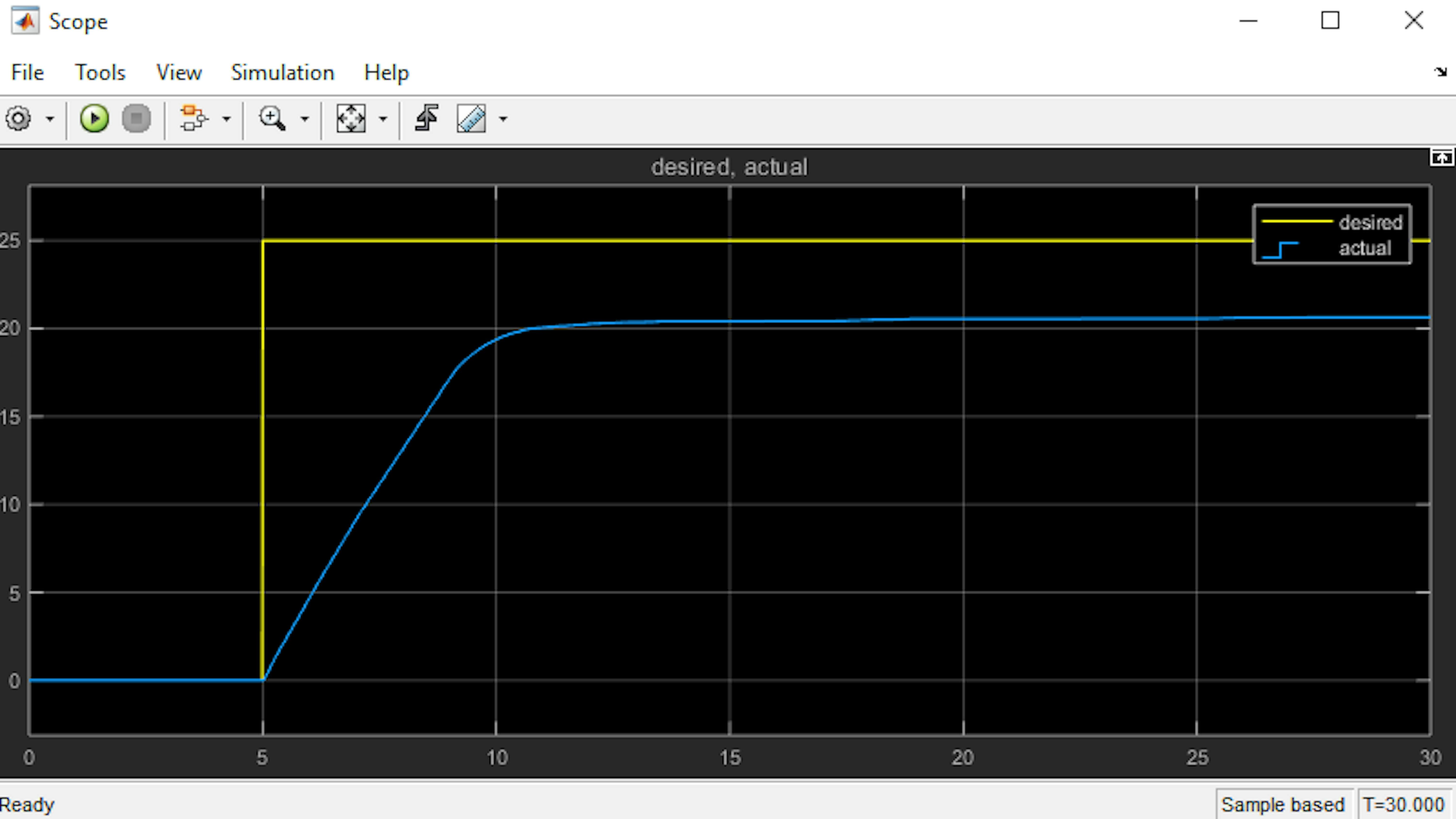
This increased the rise time to 9 seconds while also significantly increasing the steady-state error, which is defined as the difference between desired and actual values of a variable once the system has reached an equilibrium.
Note: equilibrium is also known as steady state.
Note: In some of our tests, we noticed that one of the motors was not spinning freely and this caused the steady-state error to be greater than 5. If this happens, you can use the learnings from above to have a different P gain that would give a better steady-state error.
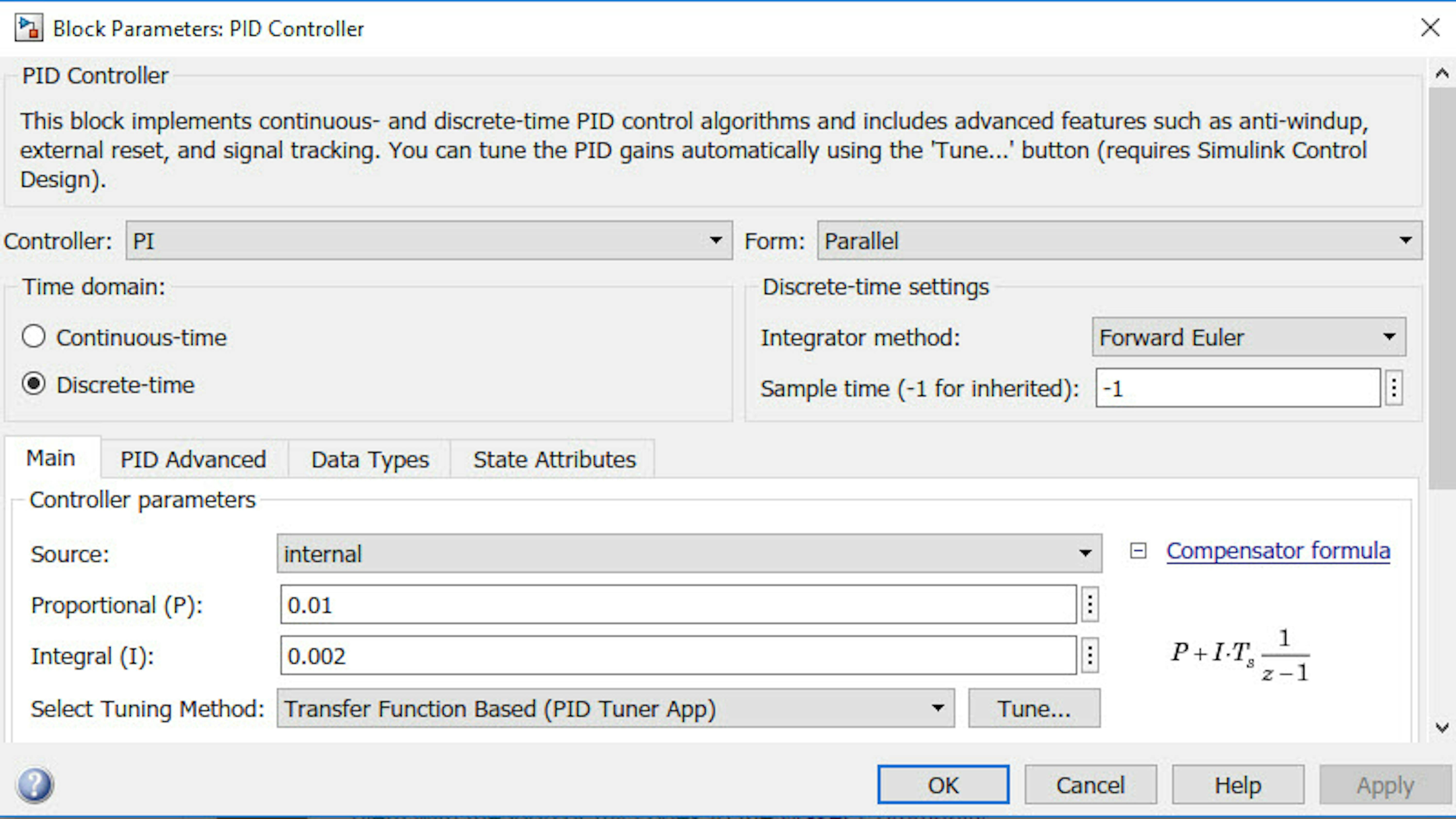
Based on the table, adding an Integral term to the controller will help to decrease steady-state error. Open the PID controller block, select PI in the Controller drop-down list and enter an integral gain value (I) of 0. 002. It is a good rule of thumb to always make sure the P value is higher than the I value.
Click Apply, and then click Run your Simulink model. Your scope should look like this.
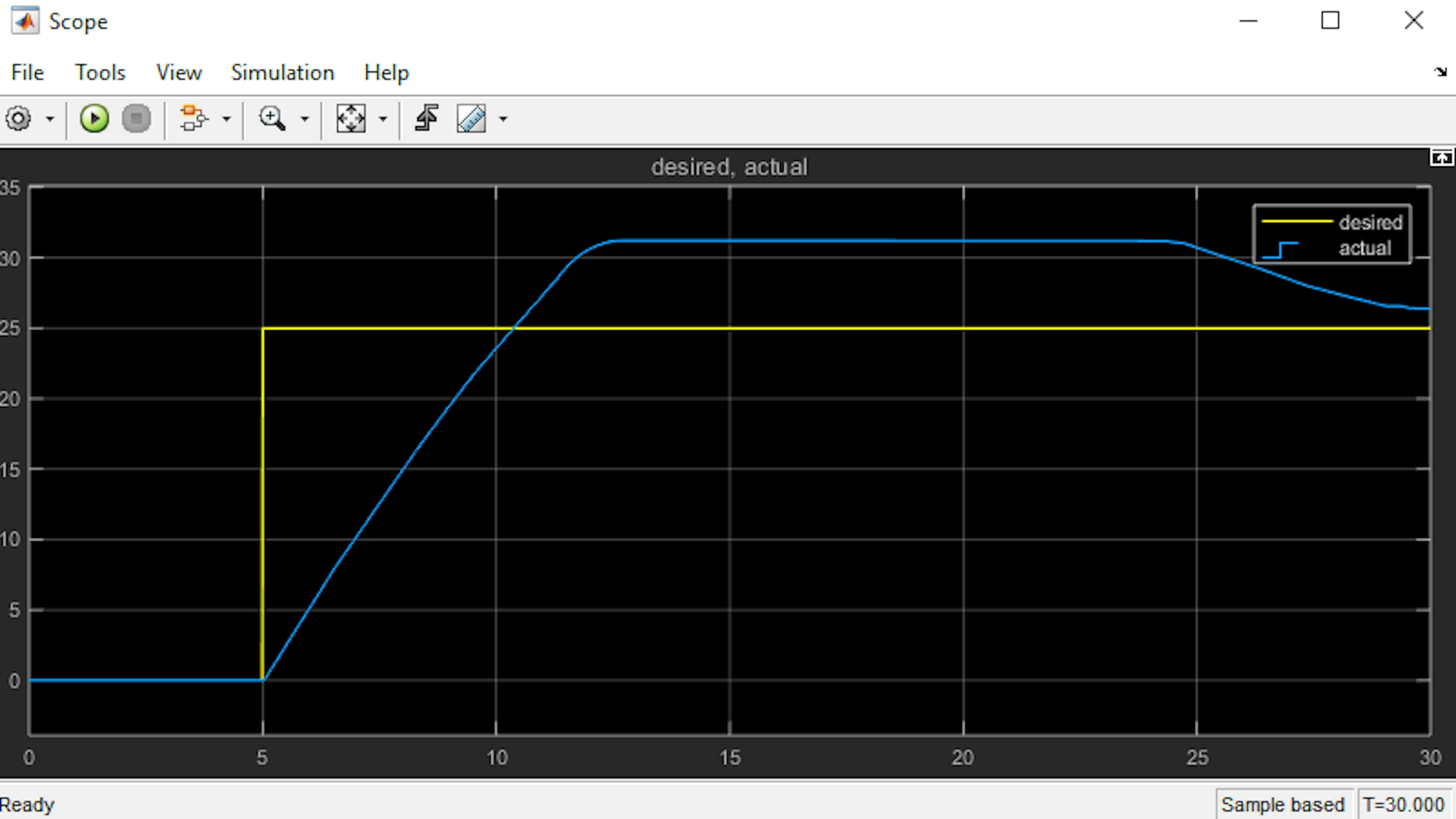
Introducing the I gain reduced steady-state error significantly, but you can see that it introduced yet another effect, called overshoot. This overshoot is measured to be roughly 6 cm. This is undesirable in our case, as the rover would go past the target location and then oscillate as it attempts to correct its position.
Referring to the table, to eliminate overshoot you can increase the P and I values.
Try increasing the P and I values using trial and error until you achieve a good balance of rise time, steady-state error and overshoot in your model.
Now, disconnect the USB cable connected to the PC and move your rover to the floor to check how the controller performs. Connect the battery and measure how far it moves. Does it move the expected 25 cm?
You're likely to find that it does move the 25 cm, but you need to adjust the PID values to account for the new operating conditions (i.e., wheels are not free-spinning when placed on the floor). The exact values will depend on the surface you use, but in several tests on relatively hard, carpeted surface it was found that P = 0.2 and I = 0.001 provided a good starting point. In some tests, these values gave an overshoot and steady-state error both around 0.2 cm.
In the next exercise, you'll see how to eliminate overshoot and steady-state error using logic-based programming and state transitions.
Note: In some of our tests, the rover never moved in a straight line and this is because of the difference in motors. You will learn how to address this issue in the next exercise.
CONTROL THE ROTATION ANGLE OF THE ROVER USING A PI CONTROLLER
This section is complementing the previous one that was looking at the rover moving over a line for a certain distance in a predetermined amount of time. In this case, you will focus on getting a similar level of control on the rover's rotational movement.
Earlier in this exercise you saw the equations to convert encoder degrees to the distance traveled:
$dr=\frac{ 2\cdot \pi \cdot r \cdot RWD}{360};dl=\frac{2\cdot \pi \cdot r\cdot LWD}{360}$
The equation to obtain the angle moved by the rover is:
$angle=\frac{dr-dl}{L}$
To design the PI controller for rotation angle of the rover, you can use the same approach that was used for controlling the distance moved by the rover. Open the model called angleClosedloop_hw:
>> angleClosedloop_hwYou can see the analogy between this model and the previous one. In this case, the linear velocity is kept constant (zero) while the rate of rotation is being controlled with the PID Controller block. This time instead of having the distance as the input, it is the rover's angle that is considered; this data is also obtained from the encoder sensor using the equation above. If you would like to understand more about how the data is being captured, open the Actual angle subsystem and explore.
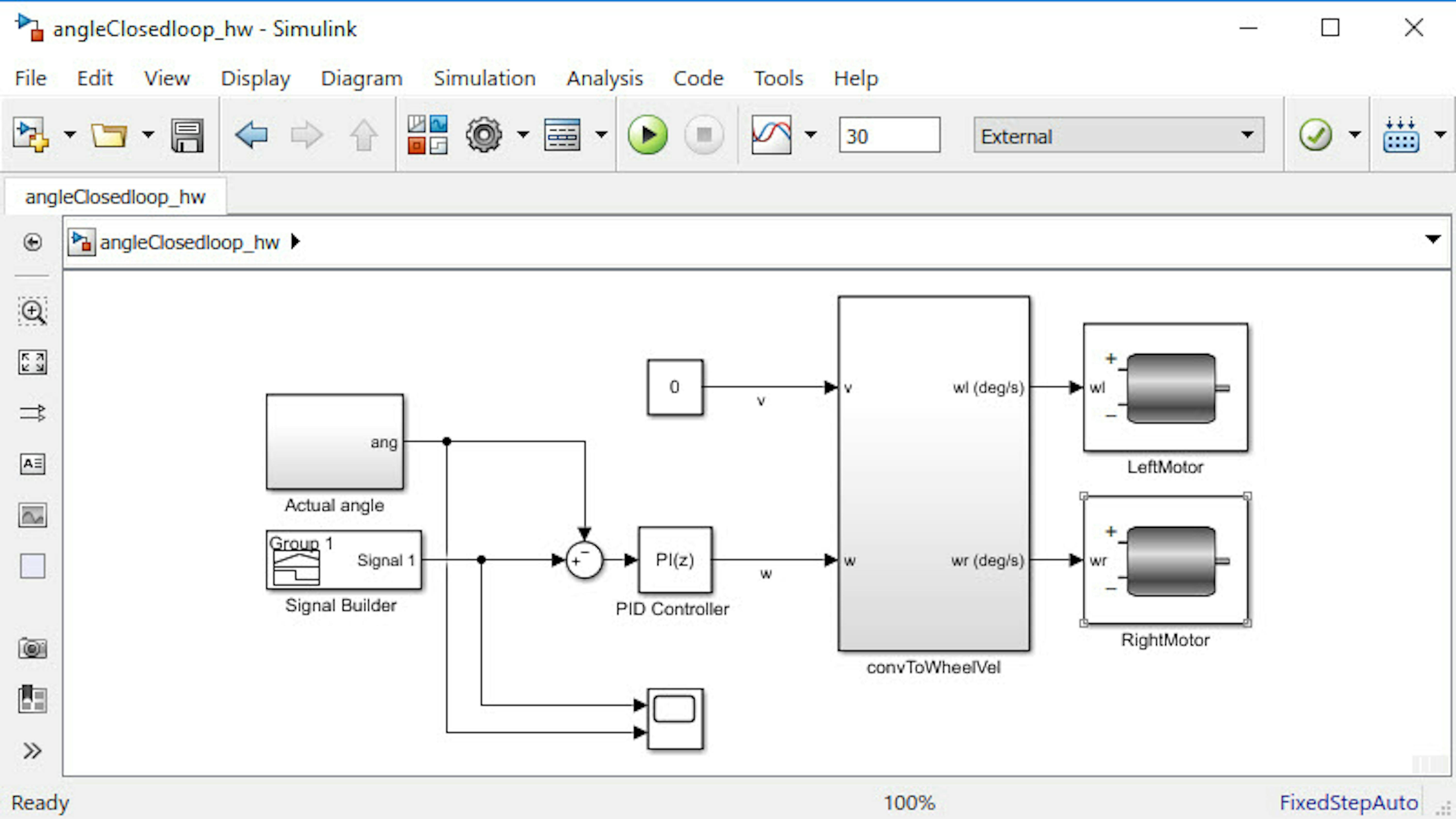
Open the PID Controller block and note the PI values. These values of P = 3 and I = 1 were a good starting point during the tests we performed when designing the experiment. In our case, the rover was moving on a relatively hard, carpeted surface. When deployed, the rover should rotate in a circle about itself and attempt to reach 90 degrees.
Run the model with your rover on the floor and tune the PI values as needed until you're satisfied with the performance within the circumstances of your experimental setup, just as you did in the previous section.
REVIEW/SUMMARY
-
We saw how to design PID controllers to control the position and angle of the rover.
-
We saw how to use external mode to tune the P, I and D gains by trial and error in Simulink and monitor the results using the Scope block.
FILES
-
distanceClosedloop_hw.slx
-
angleClosedloop_hw.slx
LEARN BY DOING
Implement a PID controller and understand how the differential term affects your controller performance on different surfaces.
EXCERCISE 4
5.4 Program Rover to follow path intructions
Now that you've learned how to implement a closed-loop PID controller on the rover, let's see how to make the rover follow a sequence of path instructions. Simulink and Stateflow will be used to instruct the rover to move forward a specified distance and turn a specified amount. We will also see how state logic can eliminate undesired effects like steady state error and overshoot of your controller.
In this exercise, you will learn to:
- Use states to program your rover to follow a sequence of path instructions.
- Use state logic to eliminate steady-state error and overshoot of your PI controller.
- Understand State logic.
SIMULATE THE ROVER FOLLOWING A SEQUENCE OF PATH INSTRUCTIONS
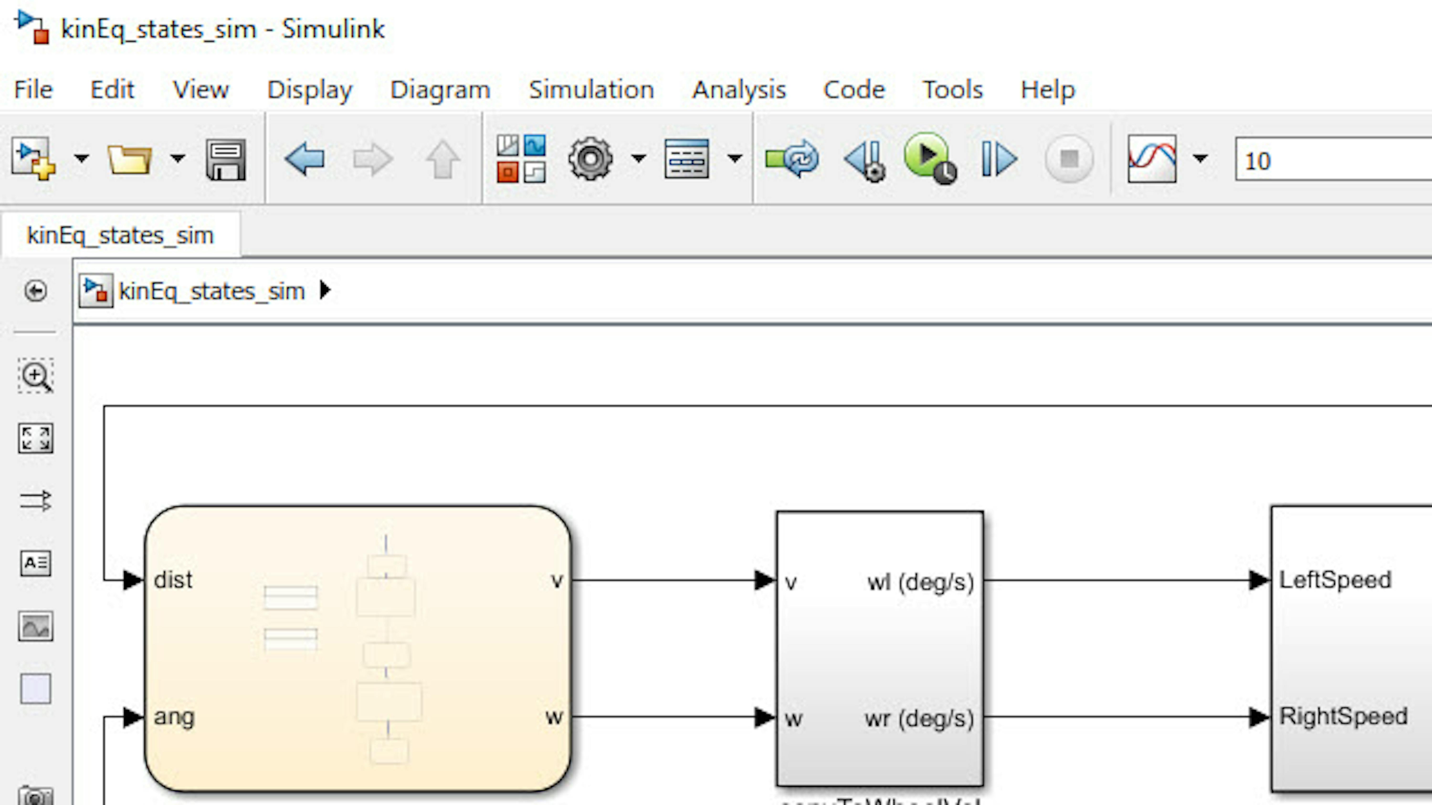
For you to start experimenting, a model including the state logic needed to command the rover is provided. Start by opening the model kinEq_states_sim.slx:
>> kinEq_states_simThis model will execute a simulation of the movement of the rover. It has the convToWheelVel and Rover Simulation subsystems and the StateLogic chart. The outputs of the Rover simulation, distance, and angle are fed to the state logic in the model, creating a feedback loop.
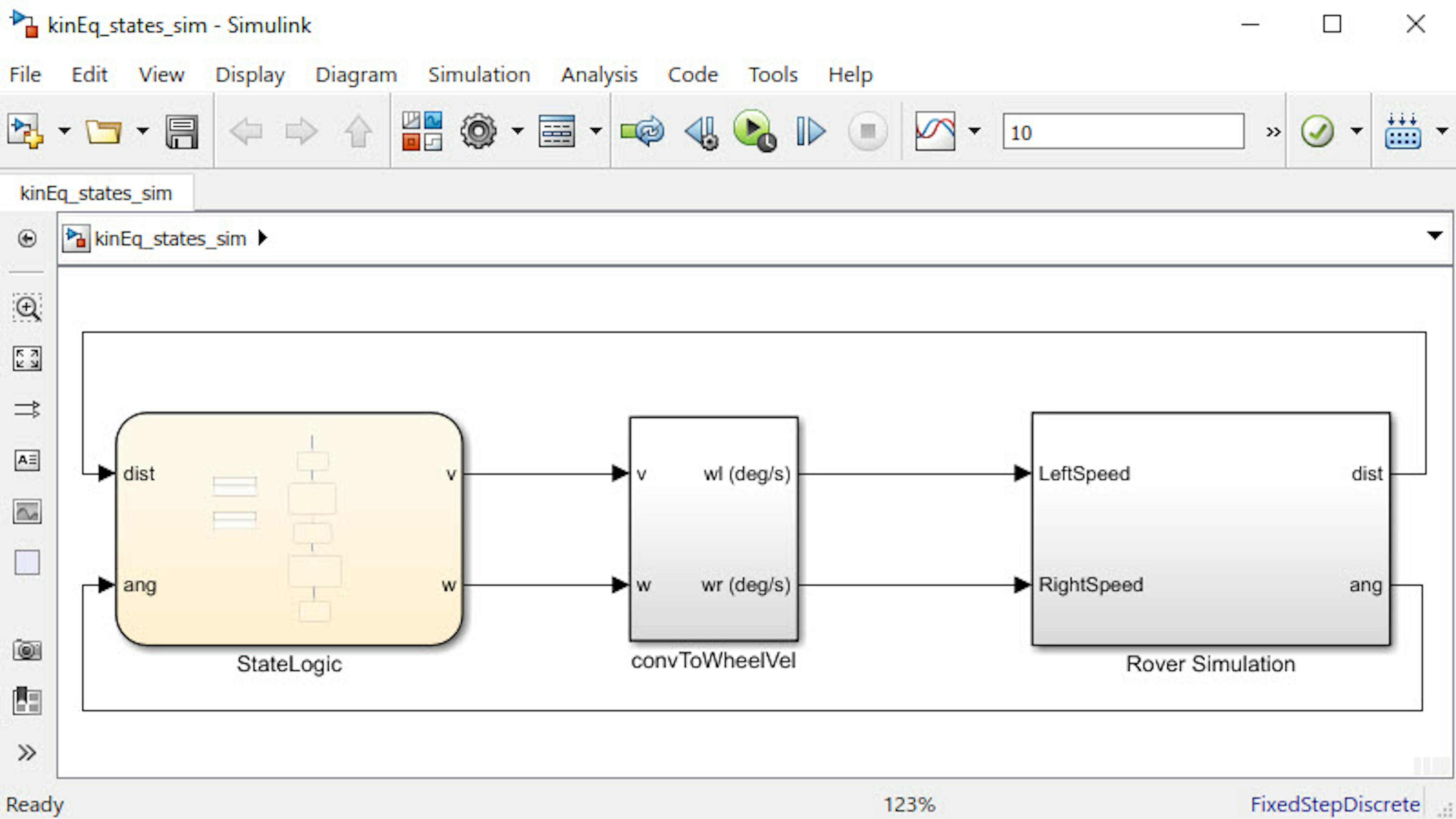
This model uses the same convToWheelVel subsystem from previous exercises to calculate wheel speeds based on desired rover velocity and rate of rotation, which will be provided by the StateLogic chart.
The Rover Simulation subsystem has one modification from the previous exercises. Its functionally is still the same, but now it also outputs values for rover distance and angle.
These values (distance and angle) are fed into the Stateflow Chart represented by the StateLogic chart, which calculates the rover's velocity and rotation rate.
Before opening the chart, you should be introduced to Stateflow. Stateflow is a software package that extends MATLAB and Simulink with tools for modeling logic and event-driven systems. This example presents key aspects of Stateflow in the context of the rover project. If you want to explore Stateflow further, you can view the Stateflow overview video and other related videos.
Open the StateLogic chart by double-clicking it. You will see a different type of block diagram where the different steps to be executed on the rover are displayed inside rounded boxes. These are called states and are displayed sequentially. They have a transition condition that is shown by an arrow at the exit of each box. These different events can be either temporal in nature (e.g., exit the block after a certain time) or boolean statements (e.g., comparing different variables against a constant).
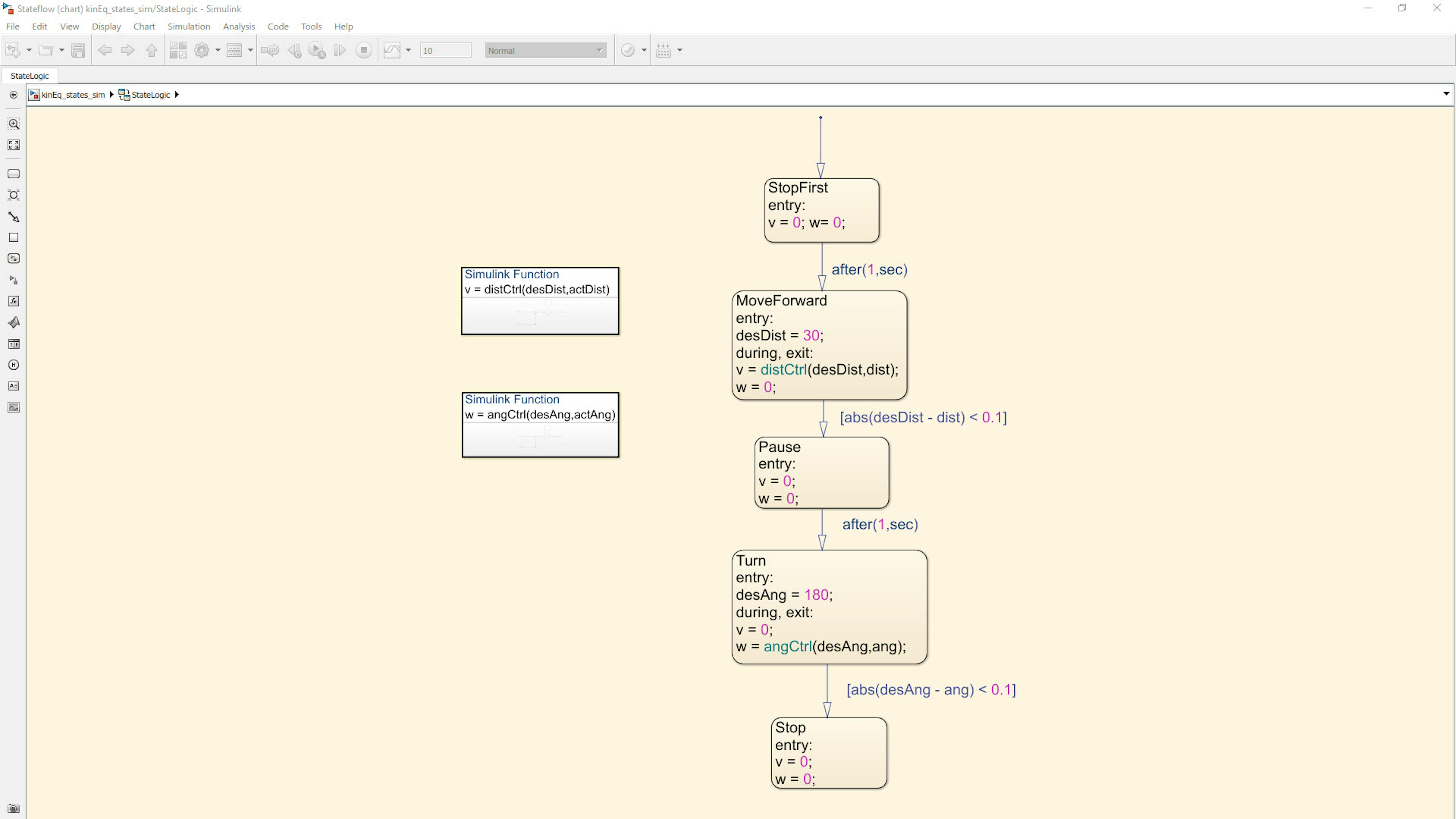
This Stateflow chart has five states that each correspond to an operating mode of the rover. When active, the contents of the state are executed sequentially.
The rover is in the StopFirst state when the simulation begins. In this state, the rover velocity and rate of rotation are set to zero, so the rover is not moving.
This state becomes inactive when the transition condition is met, in this case after(1, sec). The transition condition is tested at every time step of the simulation denoted by the sample time.
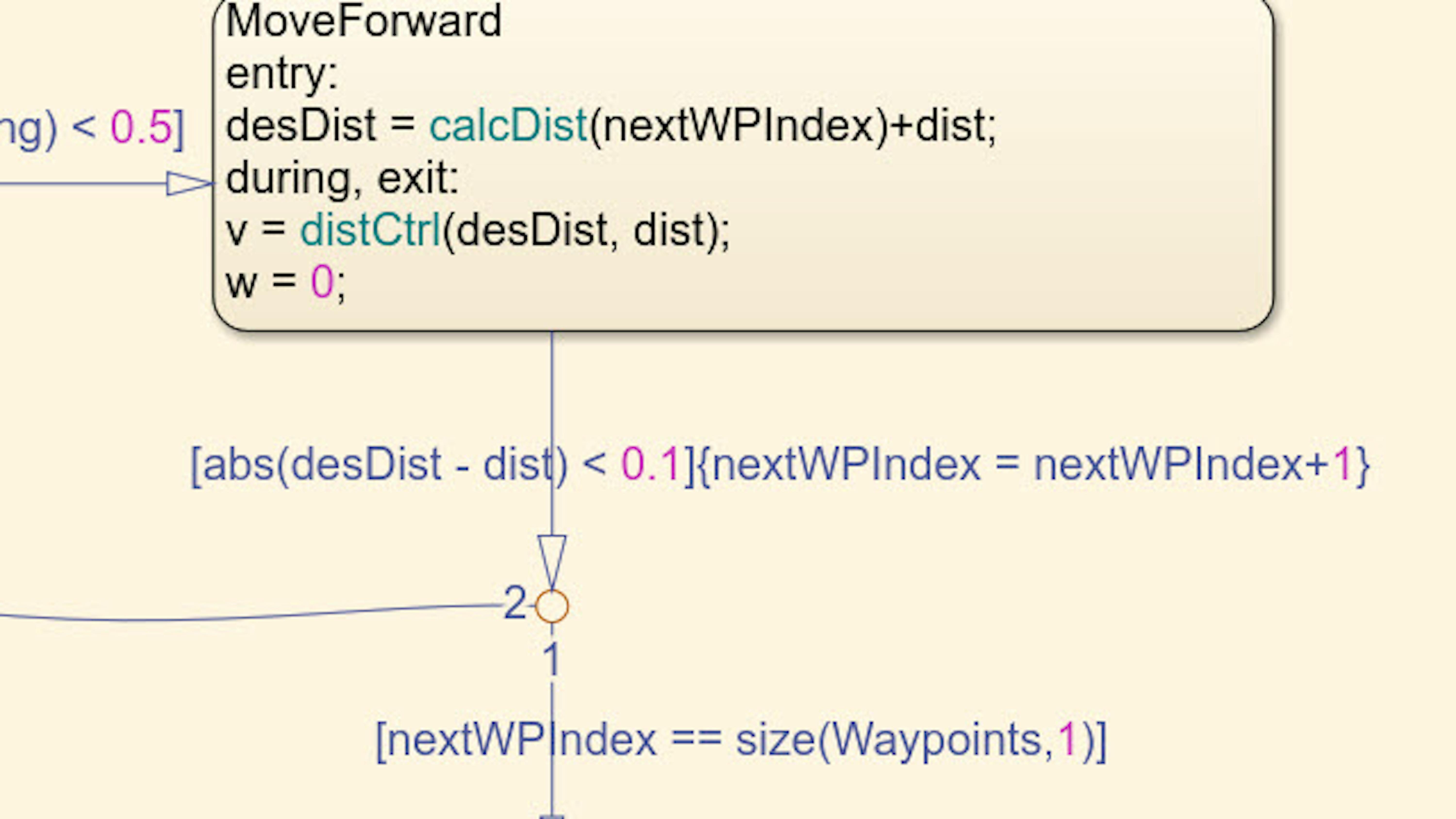
One second into the simulation, the rover transitions into the MoveForward state where it moves forward a specified distance. The entry action is executed immediately upon entering this state, and here the desDist is set to 30 cm. The entry condition can be thought of as "setup" code for each state; the entry code runs before anything else in the chart as soon as the state becomes active.
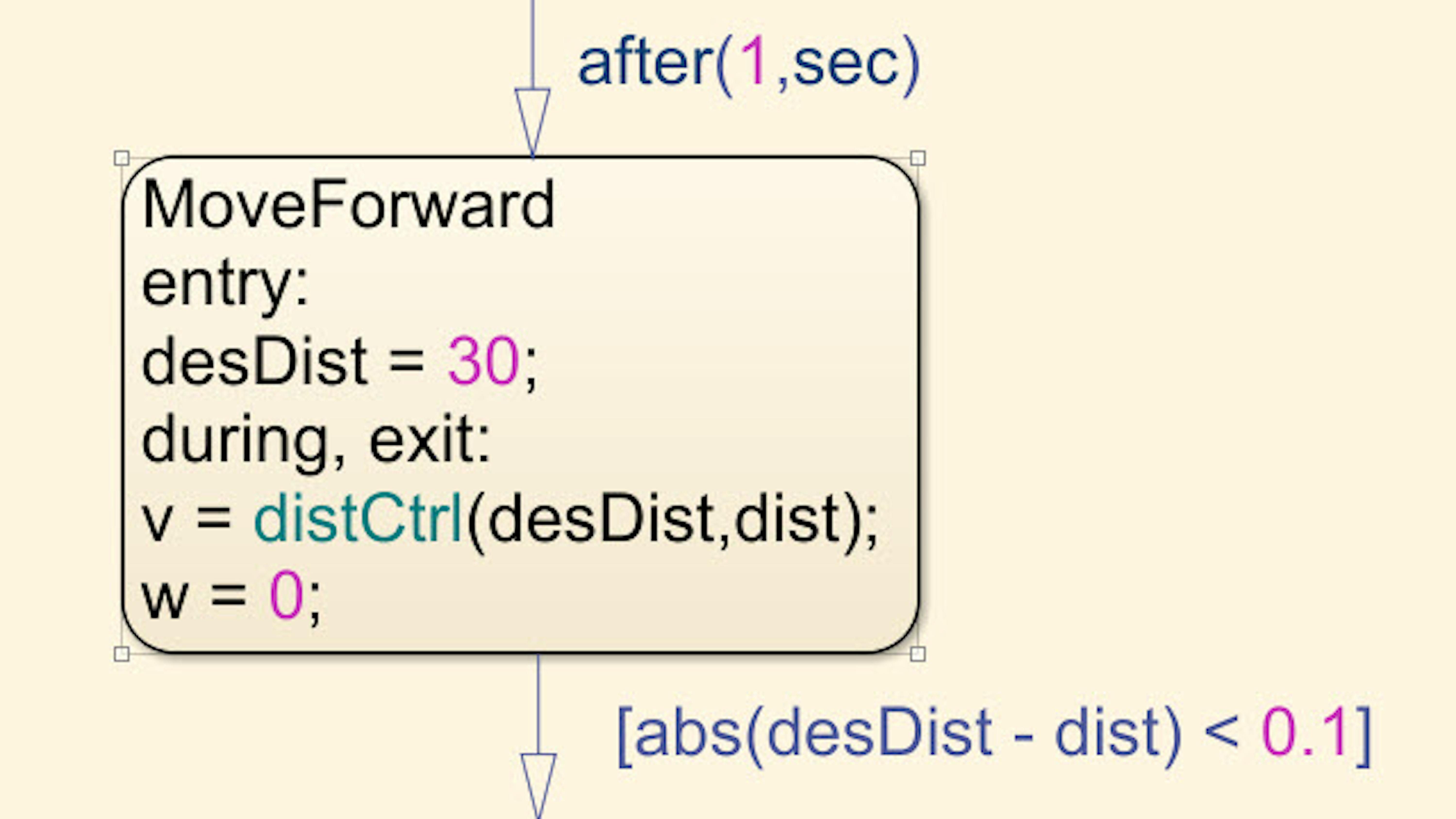
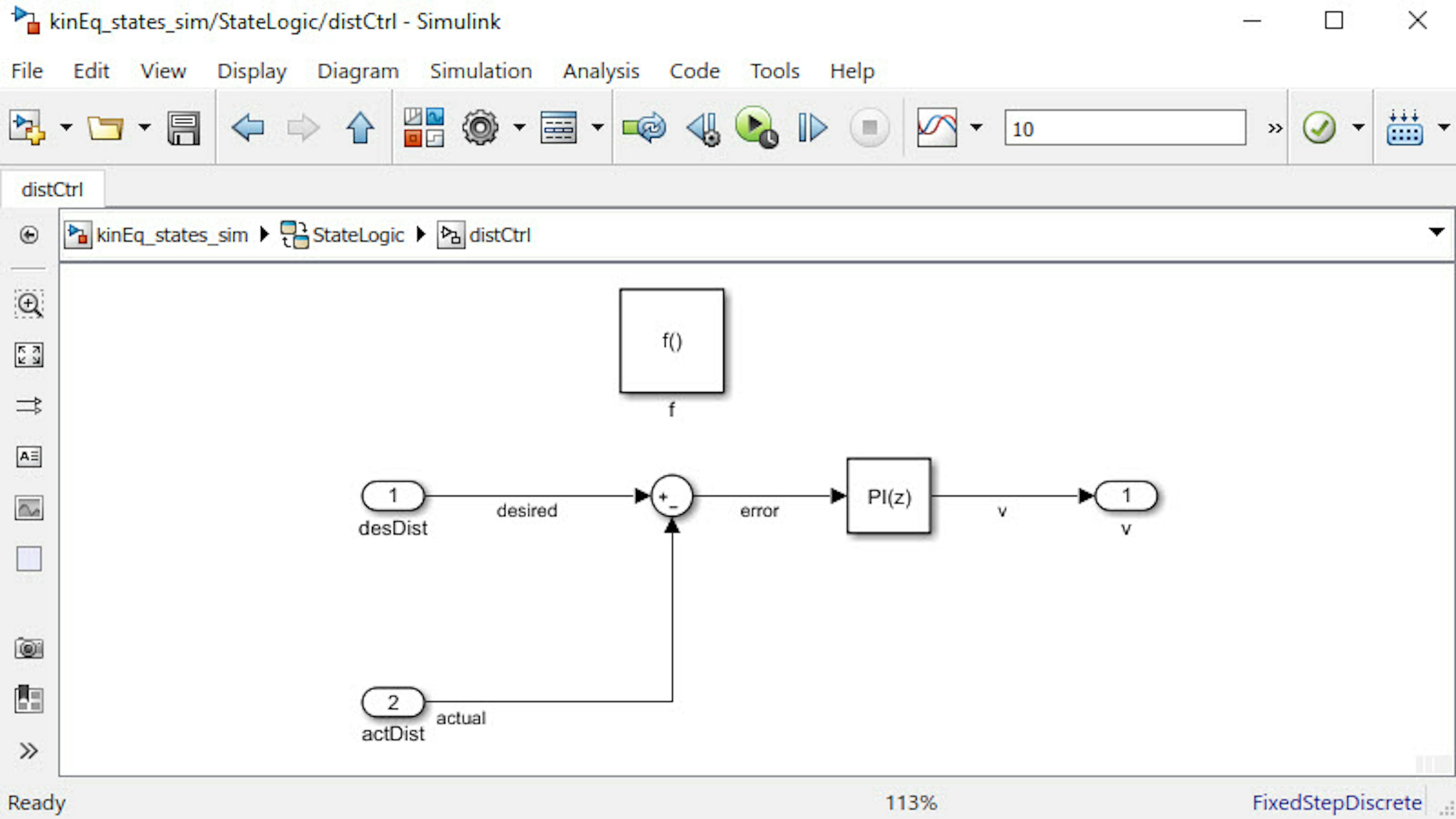
After the entry phase and for as long as this state is active, the commands in the during action are executed; the code for during can be thought of as the body of a "for" loop. Then, as the state becomes inactive, the exit commands are executed. The Simulink Function distCtrl is called, which implements the PI controller that was designed in the previous exercise. A Simulink Function is a function that is defined using Simulink blocks and it can be called at every time step from within Stateflow charts or within other Simulink models.
To transition out of the MoveForward state, the next transition condition must be met: abs(desDist - dist) < 0.1
This specifies that when the rover is within 0.1 cm of the desired distance, it should transition to the next state. Note that if your PID controller produces overshoot in the rover's distance response, it will be eliminated since the rover transitions to the next state the first time it comes within 0.1 cm of the desired distance, and any oscillatory behavior will be eliminated.
After moving forward 30 cm, the rover's next state is Pause. The rover is stationary in this state, but only for 1 second when the next transition condition is met.
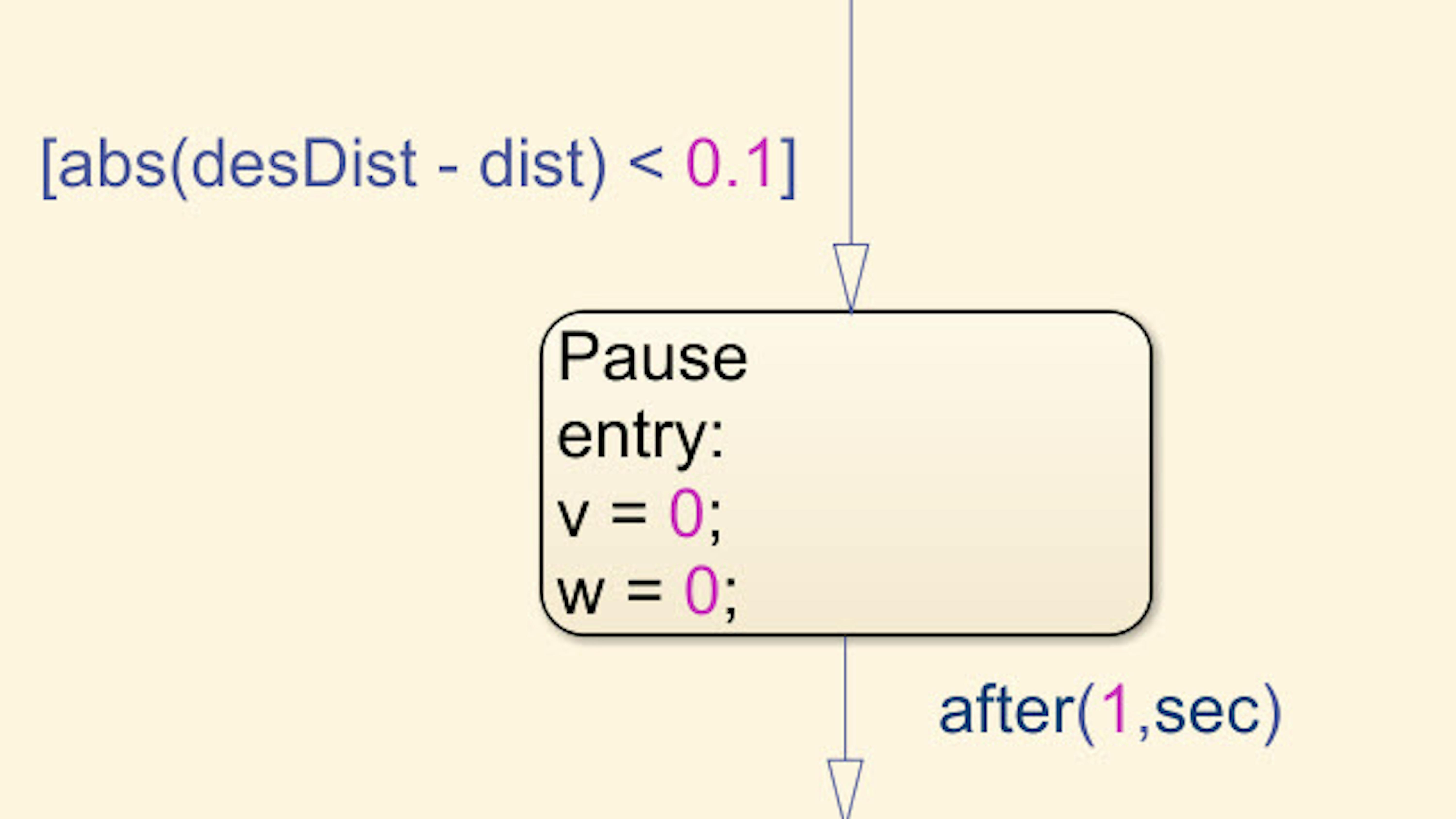
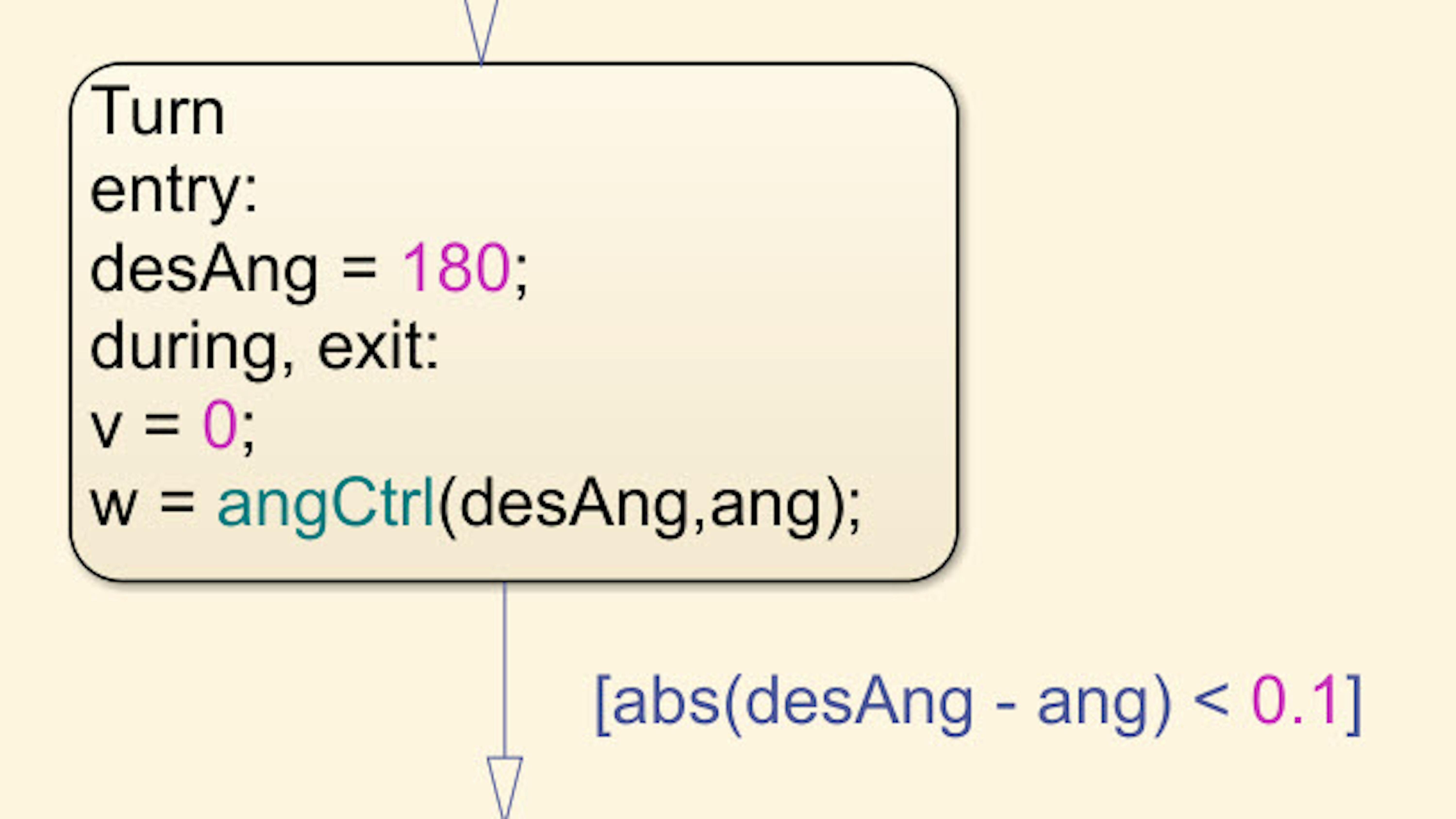
After pausing, the rover enters the Turn state. This state is like the MoveForward state except instead of moving forward 30 cm, the rover is instructed to reach 180 degrees. This state uses the Simulink Function angCtrl, which implements the PI controller that was designed in the angleClosedloophw model. Once the rover angle is within 0.1 degrees of the desired angle, the rover transitions to the Stop state.
Run a simulation of the model to see how the rover progresses through the states. Do so by clicking the Run button on the toolbar from within the StateLogic chart, as shown in the following image.
When the simulation begins, you'll see the different states highlighted as they become active.

PROGRAM THE ACTUAL ROVER TO FOLLOW PATH INSTRUCTIONS
Now that you've simulated the rover's behavior to follow the sequence of instructions, let's deploy the application to the actual rover. Connect your rover to the PC using the USB cable and Open roverClosedstates_hw.slx model by typing the following:
>> roverClosed_states_hwThis time, the model has the motors on the right side, and the angle and distance information is fed into the Stateflow chart on the left side of the diagram.
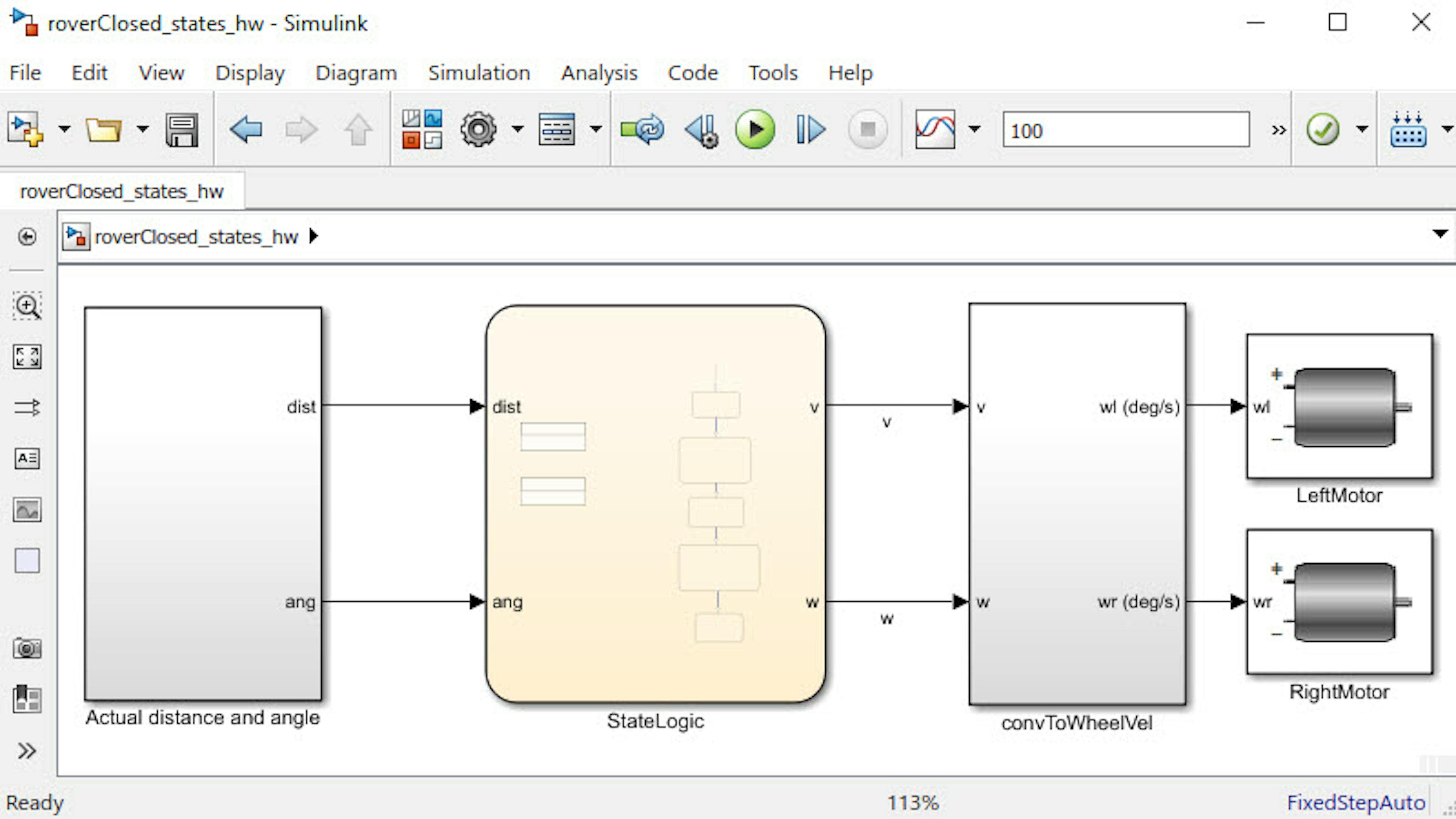
This model is like the simulation model but with a couple of key differences:
- Input to the StateLogic chart is now the rover's actual distance and angle, as measured by the encoders.
- The rotational speeds (ωl,ωr) calculated in the convToWheelVel subsystem are the input to the actual motors.
Before running this model on the rover, adjust the PI controller gains inside StateLogic to match your designs from the previous exercise.
Click the Deploy to Hardware button to download the code to the Arduino MKR1000.
Once the build process completes, place the rover on the floor and power it on using the batteries. Observe how closely your rover follows the sequence specified in the StateLogic chart.
Note: If your rover is not moving in a straight line or turning in place during those respective states, it could be because the operating conditions have changed from when you did the motor characterization experiments. You could try any of the following:
- charging your battery back to the original voltage
- Letting the motors cool off for a while
- Enabling both controllers during rover motion
We have provided a pre-built model that shows how to enable both controllers. To open this model type roverClosedBothstateshw.slx in MATLAB Command Window. In this model, explore the MoveForward and Turn states inside the StateLogic chart to understand the implementation. Remember, you can also use external mode to debug any issue that you are running into.
REVIEW/SUMMARY
-
We have seen how to use states to make your rover follow a path sequence.
-
We have seen how to use states to disable your controller, thereby eliminating the overshoot and steady-state error of the controller.
FILES
-
kinEq_states_sim.slx
-
roverClosed_states_hw.slx
-
roverClosedBoth_states_hw.slx
LEARN BY DOING
Expand the path instructions specified in the StateLogic chart and see how the rover performs.
EXERCISE 5
5.5 Localization to calculate Rover position
When working with rovers, it's often important to know their location as they move around. This exercise shows how to use a webcam with a localization algorithm to calculate the rover's location and heading. To ensure the rover remains in the webcam's field of view, the rover's movement will be constrained within a designated "arena". Start by building the arena and then perform some calibration steps to account for conditions specific to your setup (e.g., lighting, or location of webcam relative to arena). Then you will learn how the localization algorithm works and use it to calculate the rover's location and heading within the arena. This will also be used to locate the target that the rover will move with its forklift.
In this exercise, you will learn to:
- Set up and calibrate the rover's operating environment.
- Use localization to calculate the rover's position and orientation.
BUILDING AN ARENA FOR THE ROVER
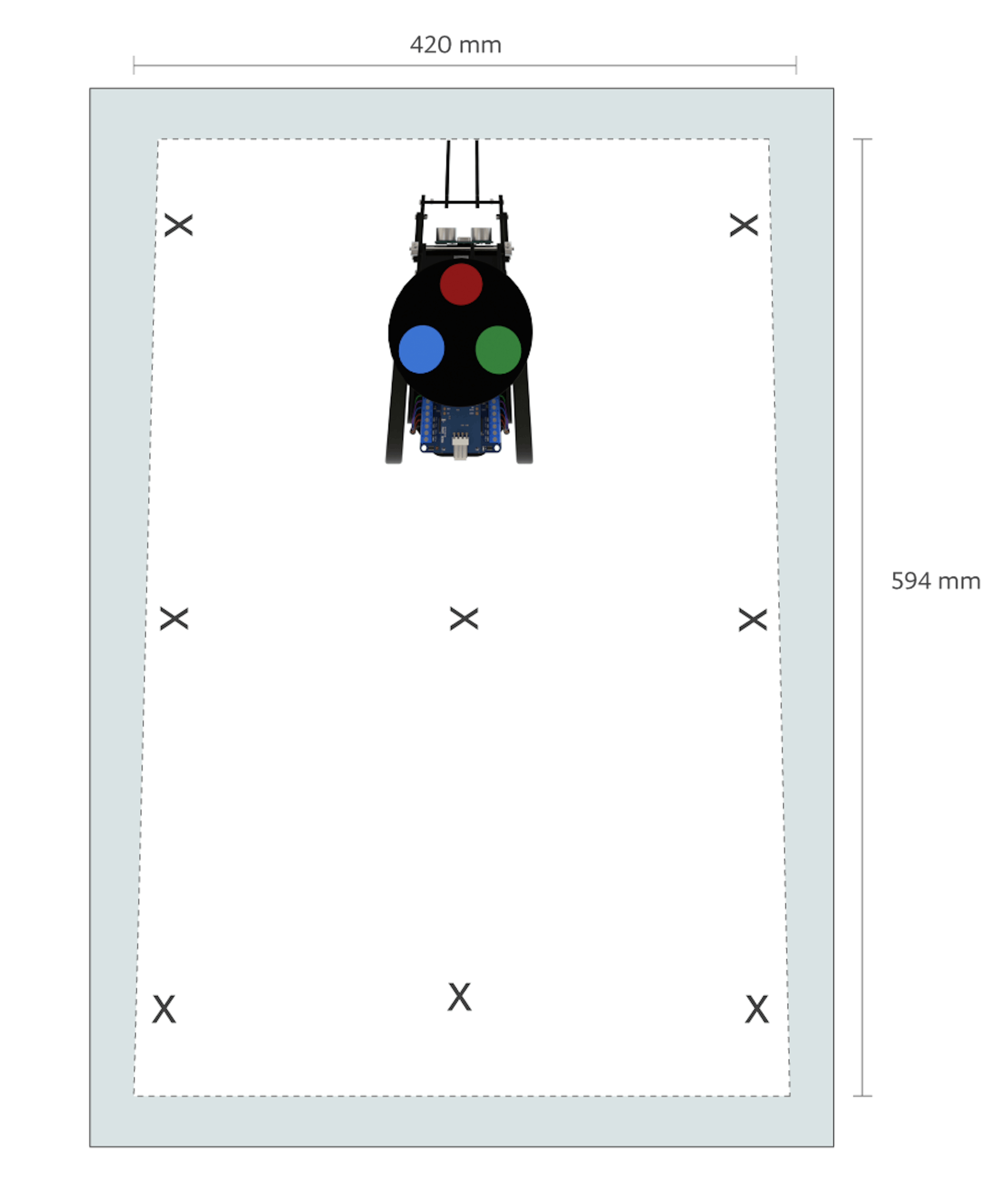
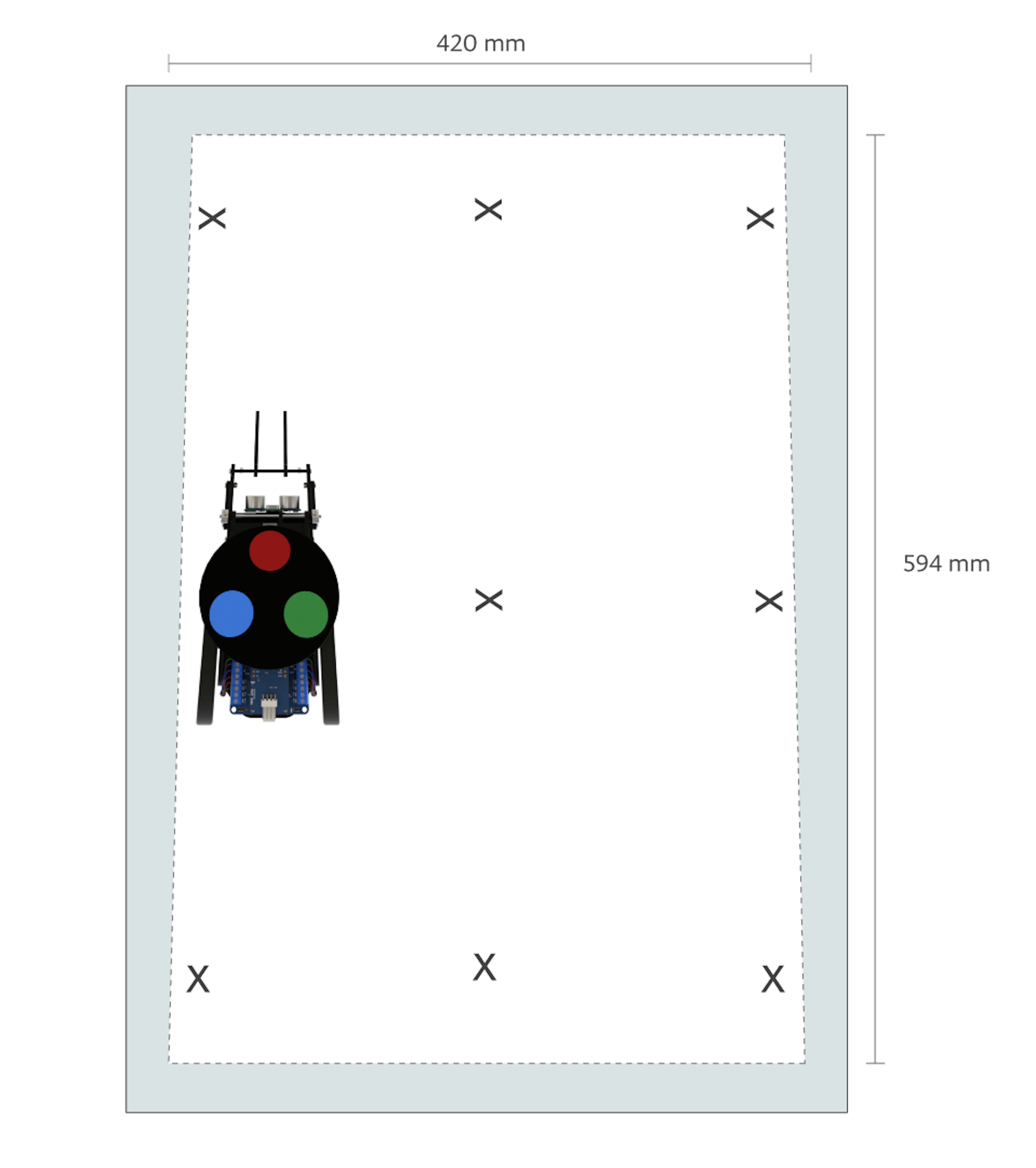
The following image shows an example arena for the rover made by using some white paper and a black marker. On the picture you can also see the rover. This can give you an idea of proportions and about how big or small your arena can be.
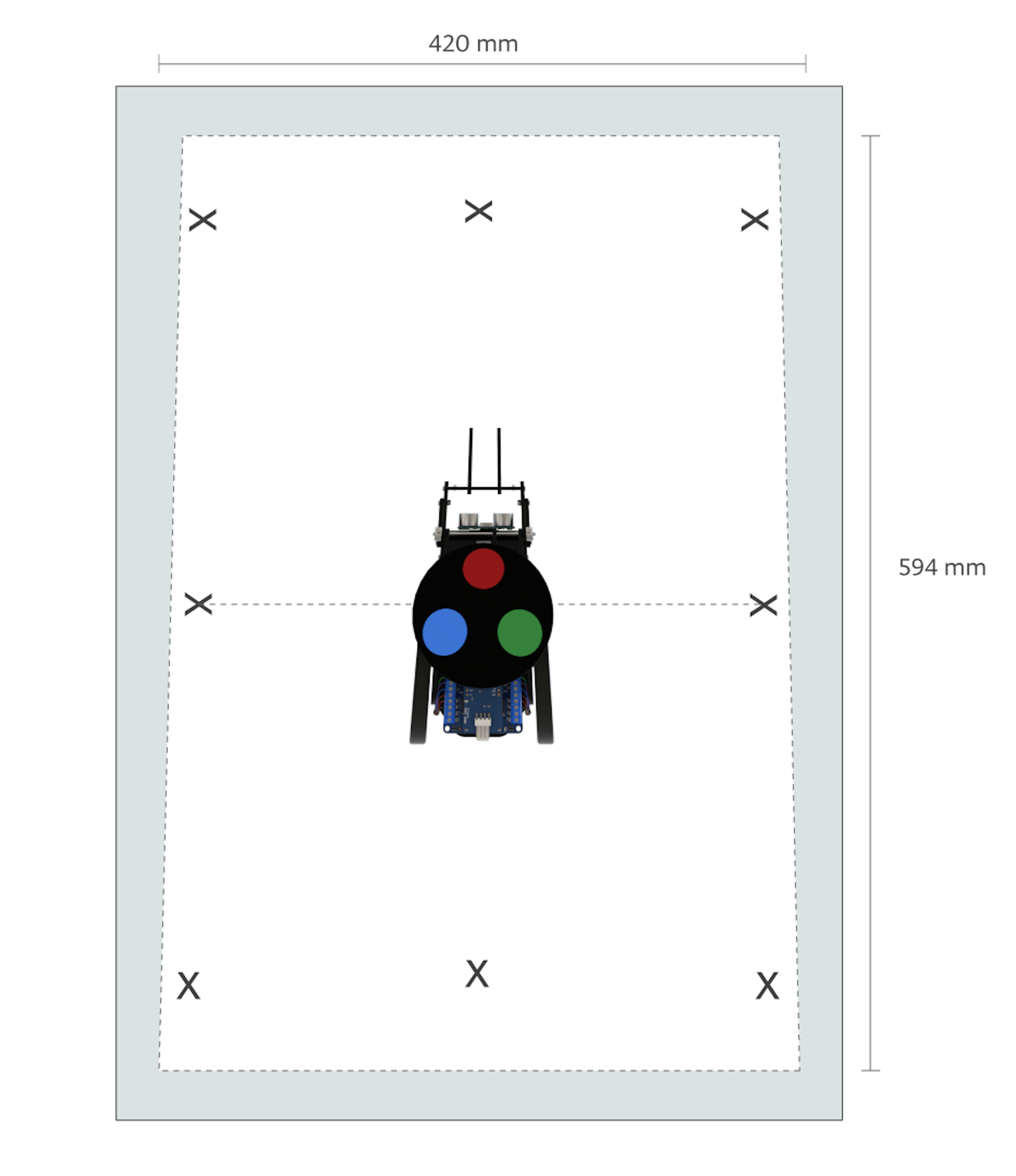
The main requirement for your arena is that it must have a white background. You can construct it using white poster board or by stapling together several sheets of paper.
The size of the arena is flexible, but it must fit within the field of view of your webcam. The localization algorithm requires that the webcam be placed at least 100 cm (approximately 3.5 feet) above the arena.
Set up your webcam over the area in which you plan to build your arena and view the video feed in MATLAB by executing the following commands:
>> cam = webcam('USB2.0 PC CAMERA');>> preview(cam)Note: You will need MATLAB Support Package for USB Webcam installed to run these commands. Refer to section 1.3.4 MATLAB and SImulink Installation
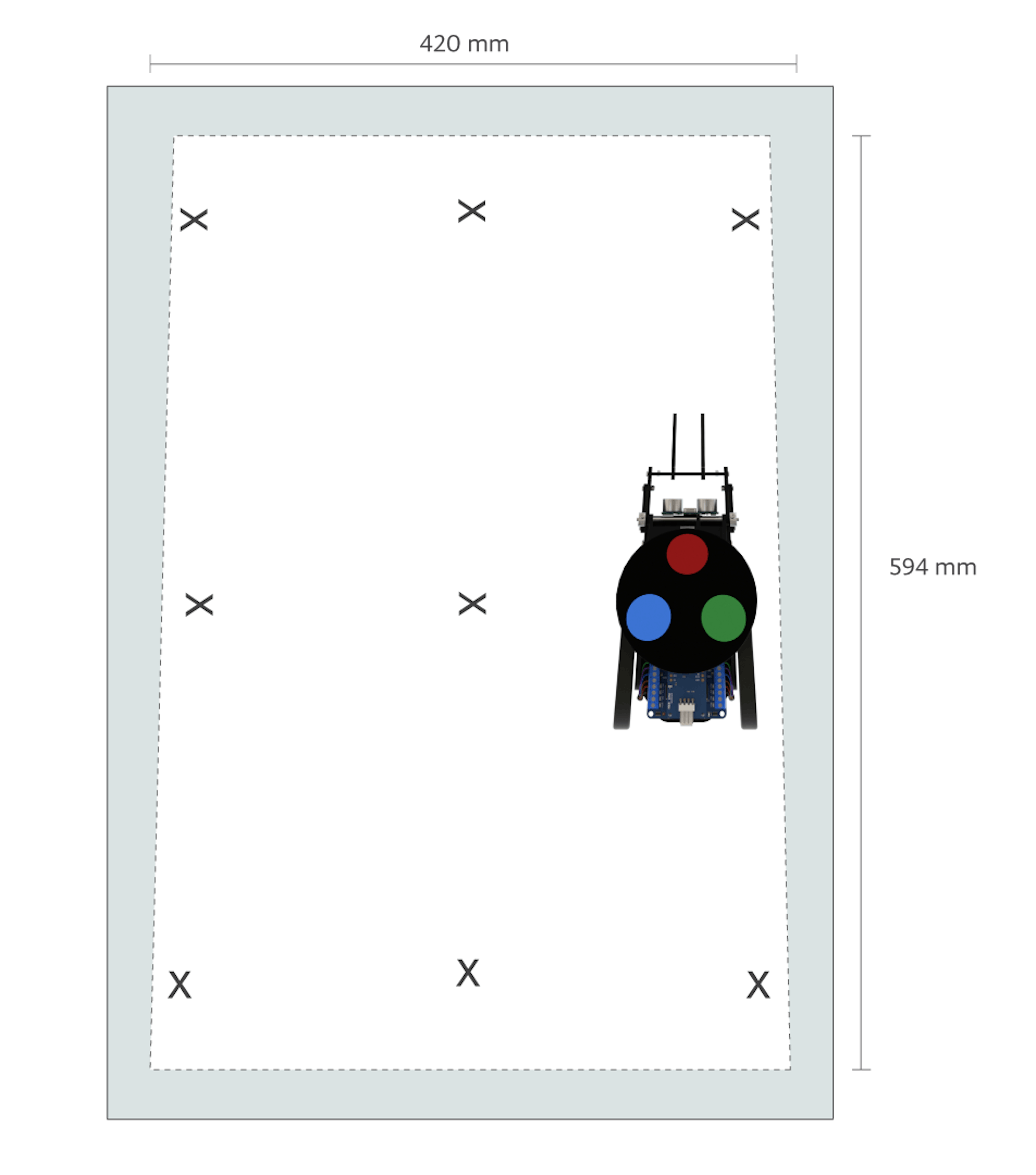
Adjust the location of the webcam and the size and placement of the arena until it fits within the field of view as shown in the image below.
You can accommodate larger arena sizes as you move the webcam farther away, but at a certain point the accuracy of the localization algorithm will be compromised. From previous tests it was found that an arena size of 75 cm x 75 cm located within 450 cm (approximately 15 feet) of the webcam works well.
When you build your arena, ensure that the white background extends beyond the actual size of the arena. Based on our experience, roughly a 5 cm padding on all sides is needed for the image processing algorithm. This will ensure that there is some buffer space between the floor and the arena.
Mark the corners of the arena, centers of all edges and the overall center point with an X that is visible from at least 100 cm away, as you saw in the picture. A black marker was used for this operation.
Confirm once again that the webcam is at least 100 cm above the arena and the entire arena is within the field of view. The next step is calibrating the image processing algorithm.
CALIBRATE THE ARENA AND ENVIRONMENT
The roverCalibration script has five steps to perform the calibration needed by the localization algorithm. Open the script and run through the steps.
>> edit roverCalibration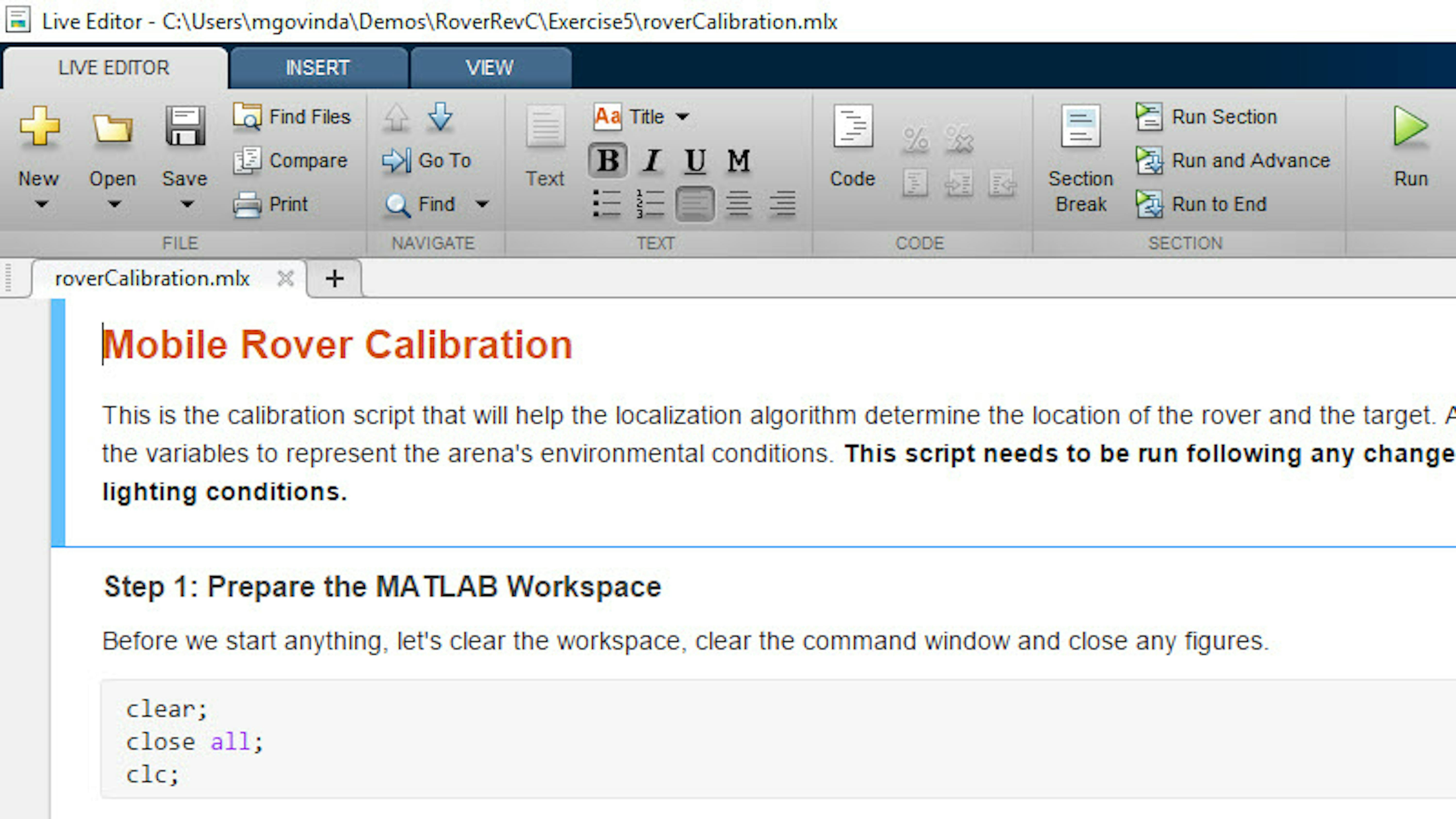
Note: The calibration process needs to be executed every time there are changes to the webcam/arena set-up, including lighting conditions. It is a time-consuming task, so it is recommended to wait until you are comfortable with your setup before running this program. Here is a step-by-step explanation of how the calibration process is performed.
The script's section called "Step 1: Prepare the MATLAB Workspace" helps clear any existing variables and close any open figures. Click Run and Advance to execute this code and move to the next section.

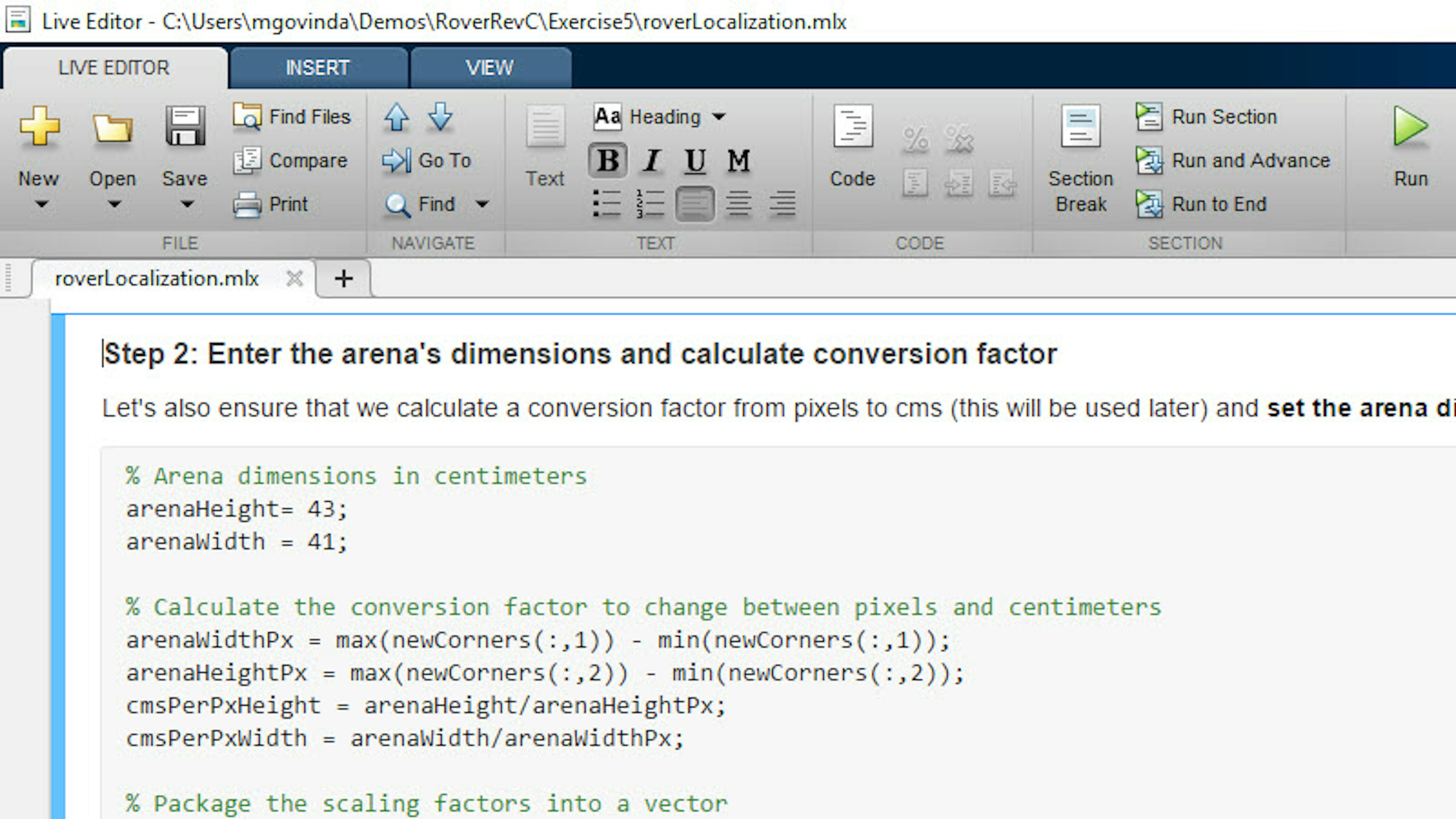
For the calibration to work, the algorithm needs to know the arena dimensions. Enter your arena's height and width in "Step 2: Enter the arena's dimensions" as shown below. Units must be in centimeters.

After entering the dimensions, click Run and Advance.
In "Step 3: Initialize the webcam and compute the transformation that gives the orthogonal view," the webcam will be initialized. Later, the transformation that gives the orthogonal view of the rover will be computed. To select your webcam, you can use the automatic suggestion feature inside the Live Script as shown below.
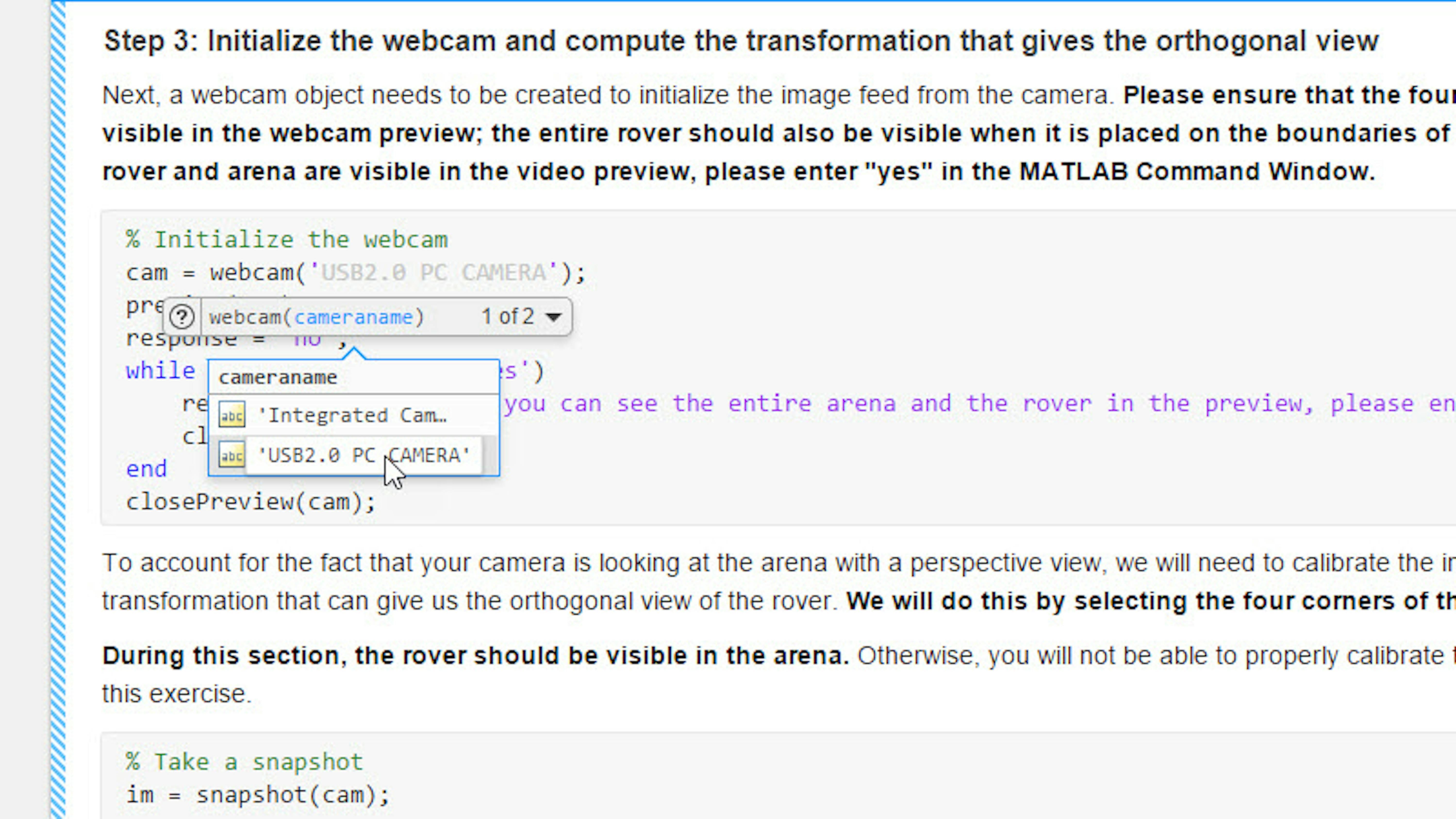
Now let's look at the transformation portion of this step. Typically, it is hard to place the webcam directly over the arena, and instead the camera is placed where it takes images from some downward angle. Image processing can be used to translate the image to a corrected version of itself, which will make it easier for our localization algorithm to calculate the position. Execute this section by clicking the Run and Advance button to see what effect this has on the image. Follow the instructions that appear in the MATLAB Command Window.

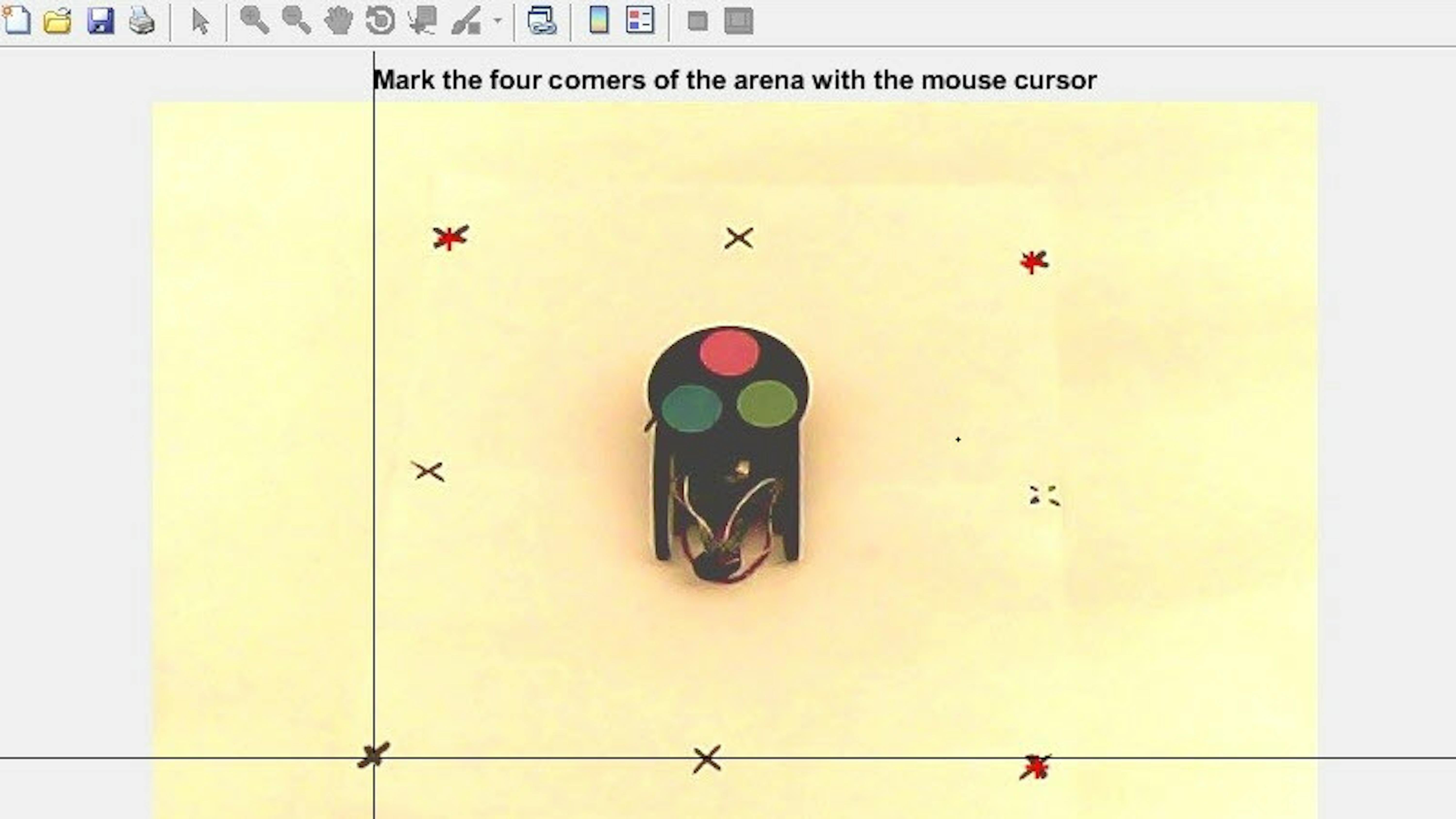
The webcam image will be displayed; to compute the transformation of the image, click the four corners of the arena in the image.
Important: Ensure that the rover is in the arena. If it is not, you need to execute this section of the code once more with the rover placed in the arena.
If you would like to look at the transformed image, execute the following command in MATLAB:
>> imshow(orthoImg)Note: It is common for orthogonally rotated images in this project to have missing portions of image. These are the black portions at the bottom of the image above.
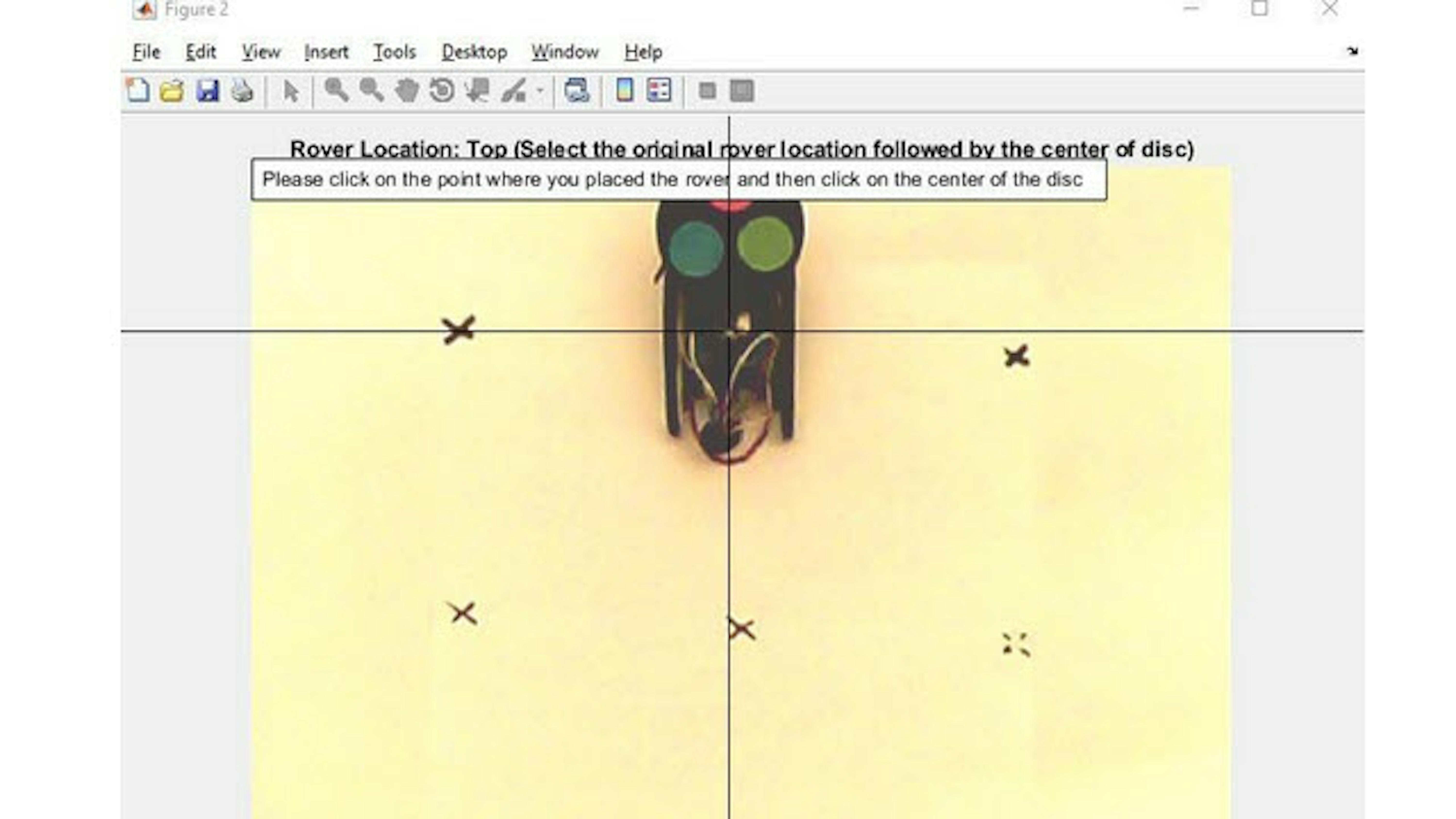
Because the webcam takes pictures from an angle, the rover's height is altered differently for various distances. Step 4 has been split into "Step 4a: Compute the location offset for the rover" and "Step 4b: Compute the location offset for the target". In Step 4a, you will capture images of the rover on the four edges of the arena (TOP, BOTTOM, LEFT and RIGHT as shown in the image series below) to account for this.
TOP
BOTTOM

LEFT
RIGHT
Run the first section of Step 4a of the live script by clicking Run Section, then place the rover as instructed in the prompts displayed in MATLAB.
In the next section of code, the calibrateLocationOffset function operates on the images that you just took. The image that pops up shows a clear visualization of how the height is translated differently for different depths from the camera. Click the points specified in the pop-up figures (center of the rover and the center of the disc) to compute the offsets.
Now let's click the section entitled "Compute the offsets of the rover" and then click Run and Advance to perform all the necessary tasks.
Next, let's repeat these tasks for the target in Step 4b. Again, click the Run and Advance button and follow the prompts displayed in MATLAB.
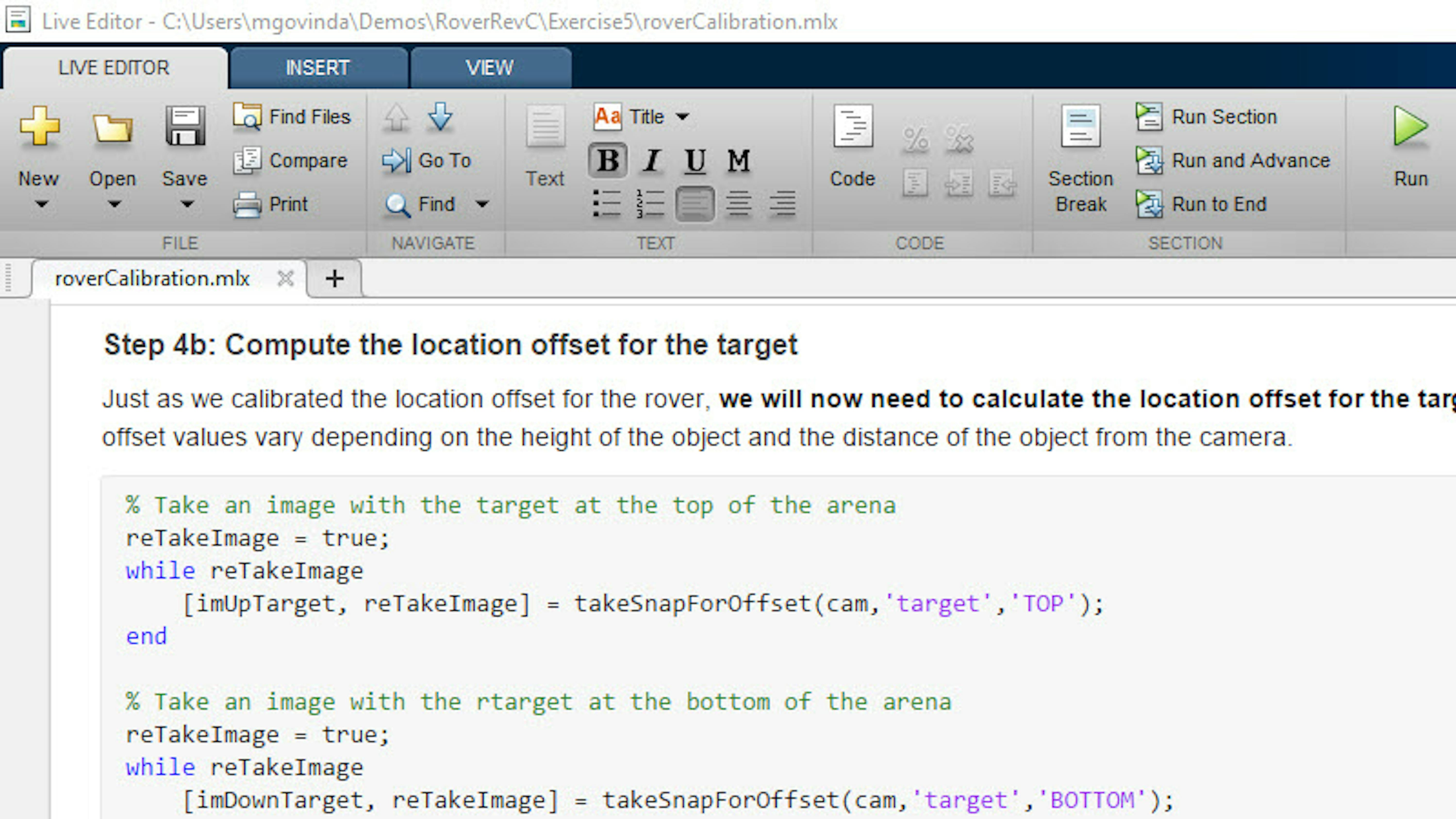
Run the next section titled "Compute the location offset for the target", where you will place the rover in different locations as per instructions on MATLAB Command Window and then click the locations where the target was placed followed by the center of the target on the image. The localization results depend heavily on these steps and can cause issues if the calibration is not done accurately. A sample image is offered in that section of the live script.
In "Step 5: Calibrate the color threshold of the disc", you will see how to account for the lighting. Click this section of the code to select it and click Run this section of code. On the image that appears, ensure that you click the circles in this order: Red first, Green next, and then Blue.
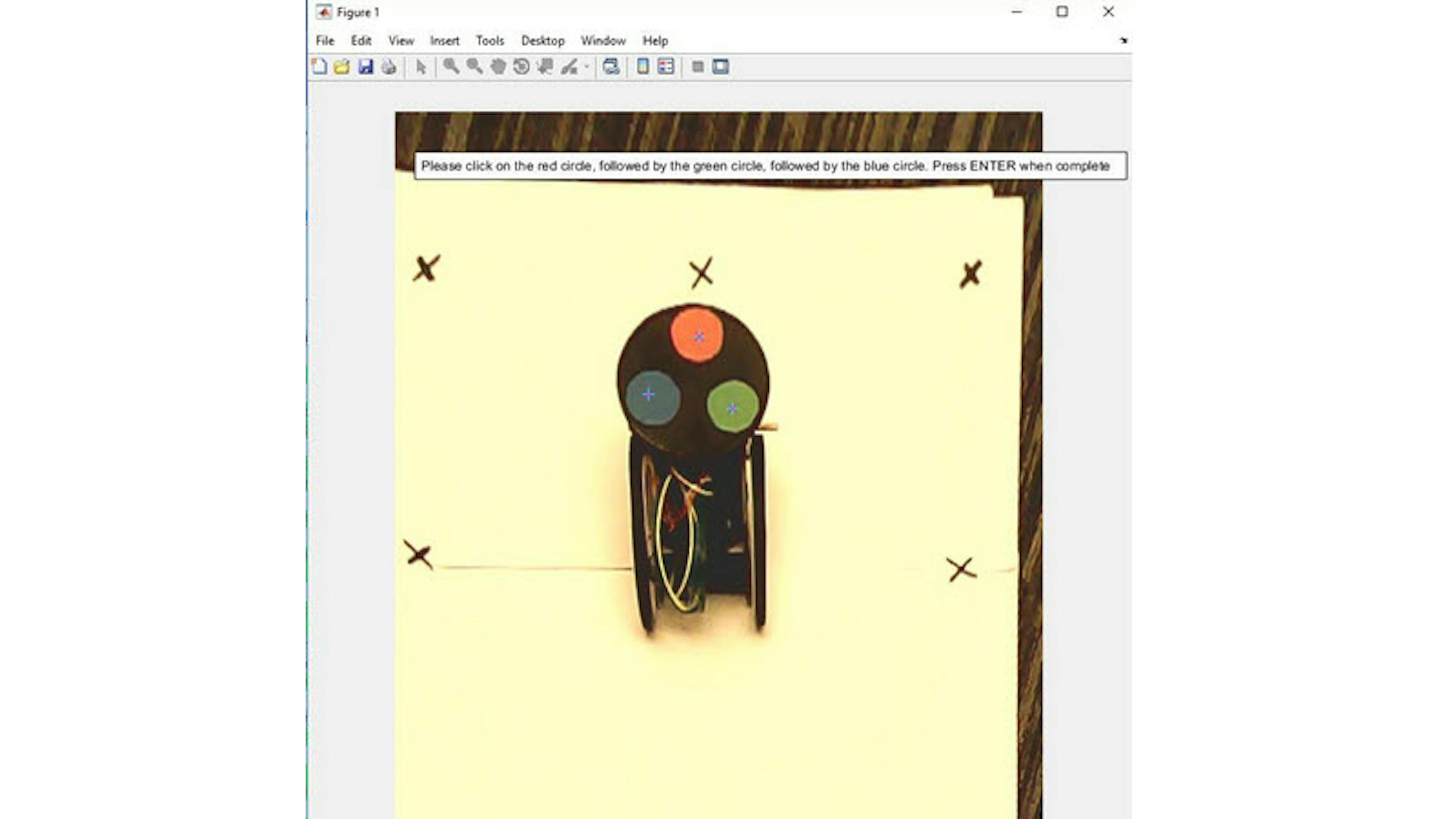
Note: Once you have clicked the circles, you should press the ENTER key to confirm your selections.
With that, you have now calibrated the parameters to get an orthogonal view of the rover, corrected for any location offsets within that view and accounted for how lighting can affect the RGB values for colors. All the calibration data is saved and will be reused during the execution of the localization scripts.
LOCALIZATION OF THE ROVER AND THE TARGET
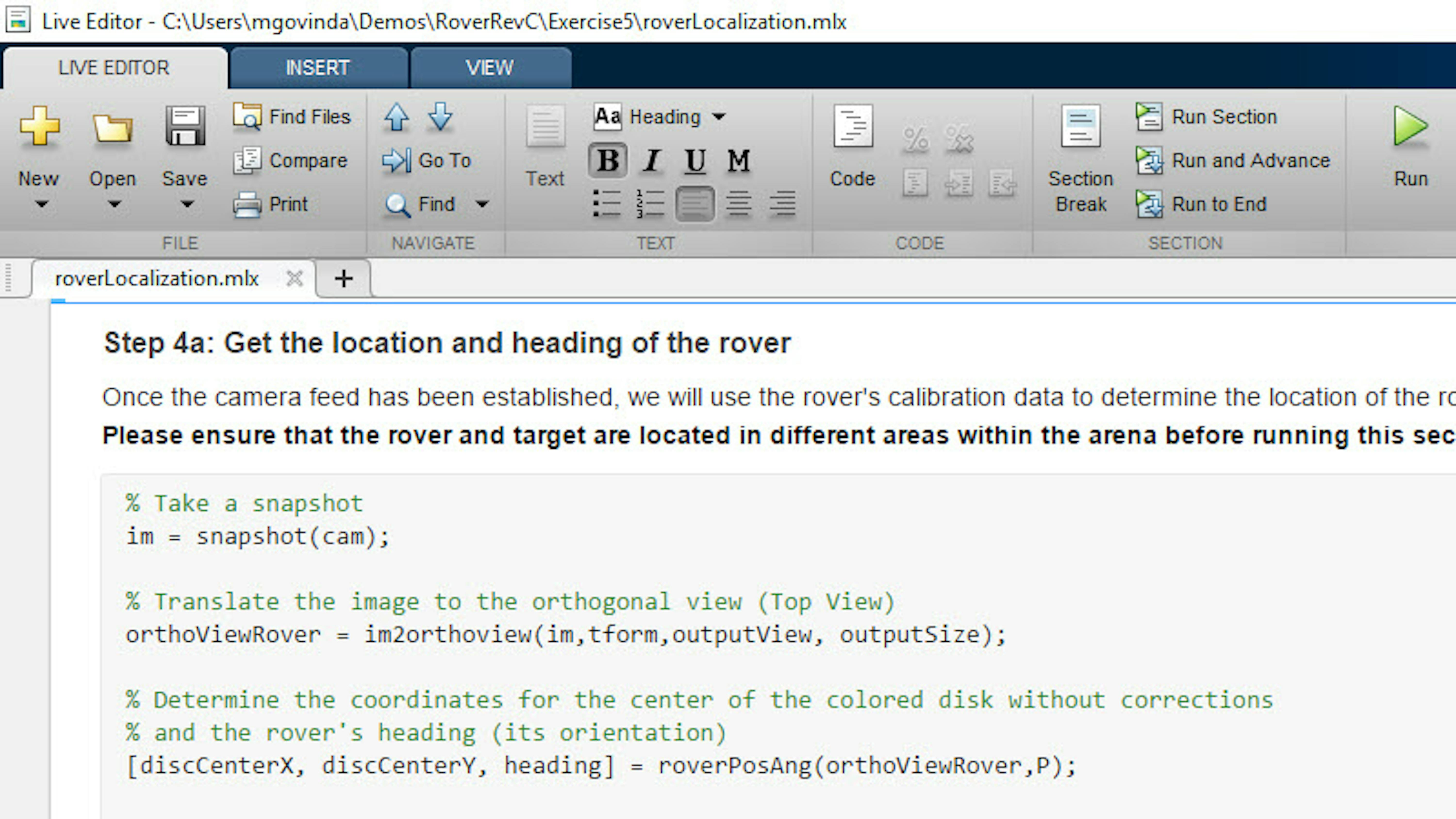
Now that you've completed the calibration, let's see how to use the localization algorithm to calculate the position and heading of the rover within the arena in five simple steps. Open the live script roverLocalization.mlx :
>> edit roverLocalization
Let's run "Step 1: Prepare the MATLAB Workspace" of this live script to clean up the Workspace and load the Calibration data generated earlier.
Enter your arena's dimensions in "Step 2: Enter the arena's dimension and calculate conversion factor" and run this section of code. The conversion factor calculated in this section relates the real-world dimensions of the arena in centimeters to the number of pixels within the image. This is achieved by dividing the physical arena measurements with the corresponding number of pixels from the image.
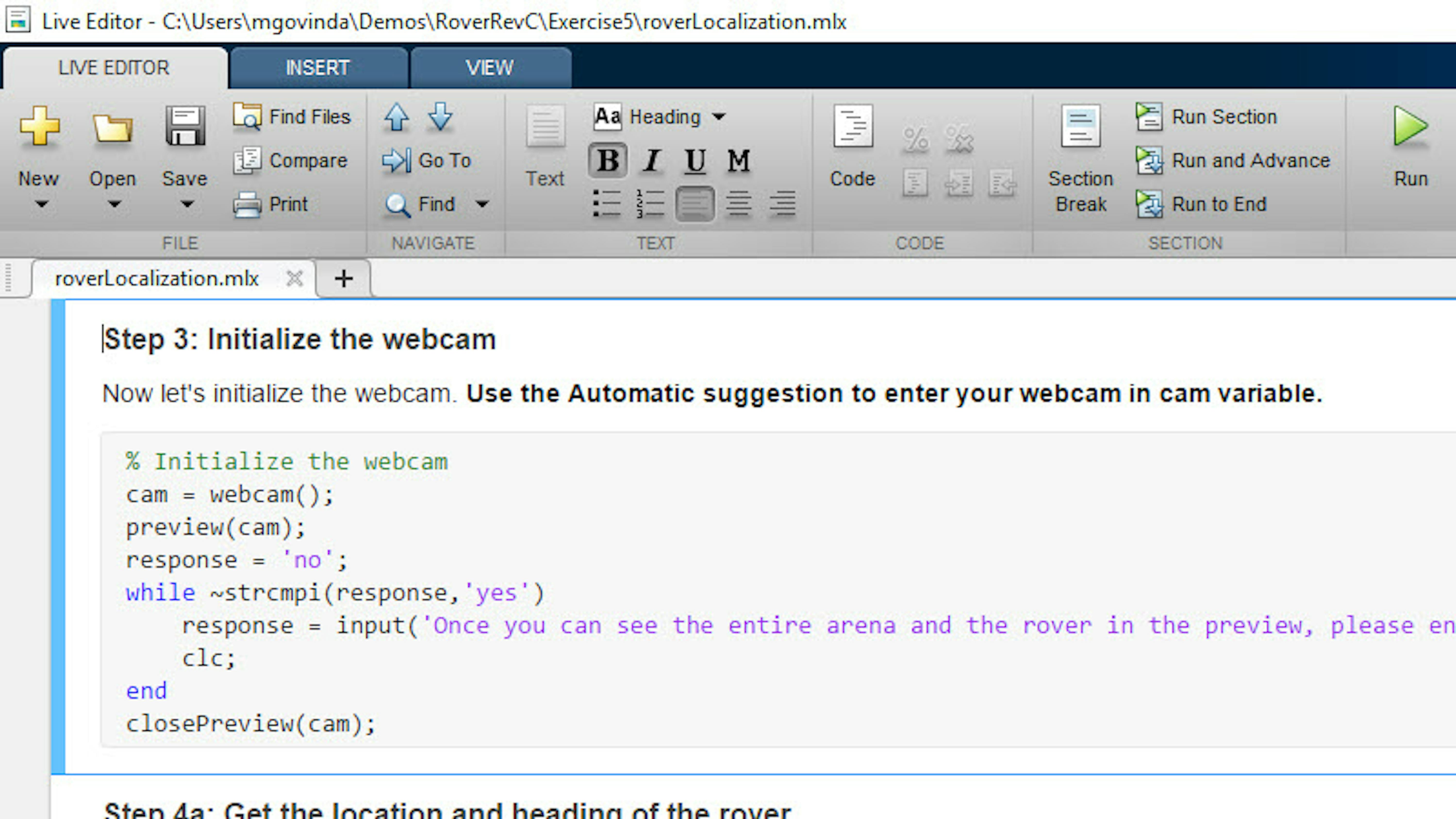
In "Step 3: Initialize the webcam," select the appropriate webcam using the automatic suggestion feature that was introduced in the previous section and run this section of code to initialize the webcam.
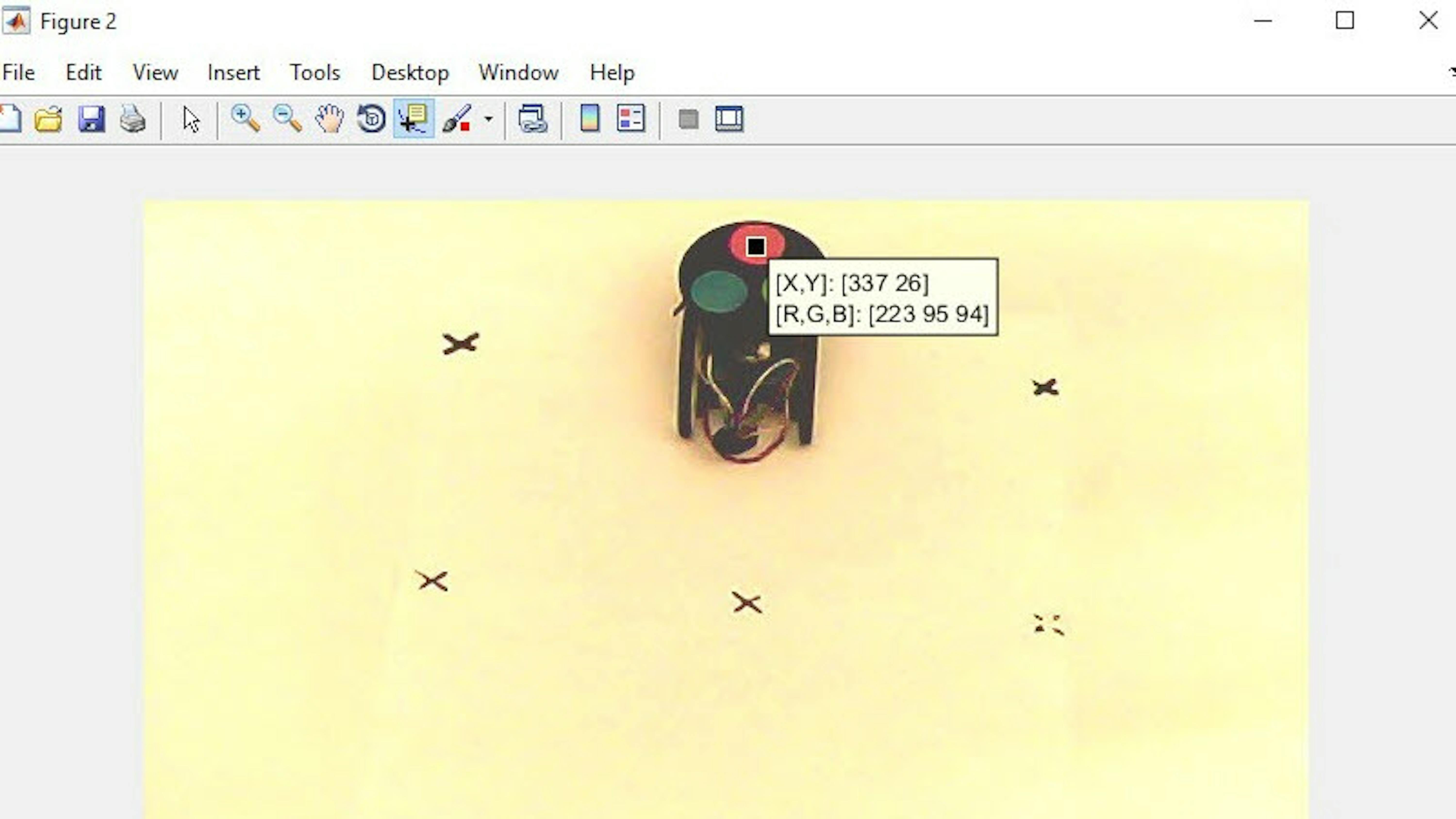
The following section, named "Step 4a: Get the location and heading of the rover," uses the calibration data to determine the location and heading of the rover within the image. Shown below is a schematic that provides an overview of the localization algorithm itself.
LINE-BY-LINE EXPLANATION: ROVERPOSANG FUNCTION
To obtain the rover position and heading from the orthogonal image, we created the roverPosAng function.
This function calculates rover position (x,y) and heading. x and y are returned in pixel coordinates.
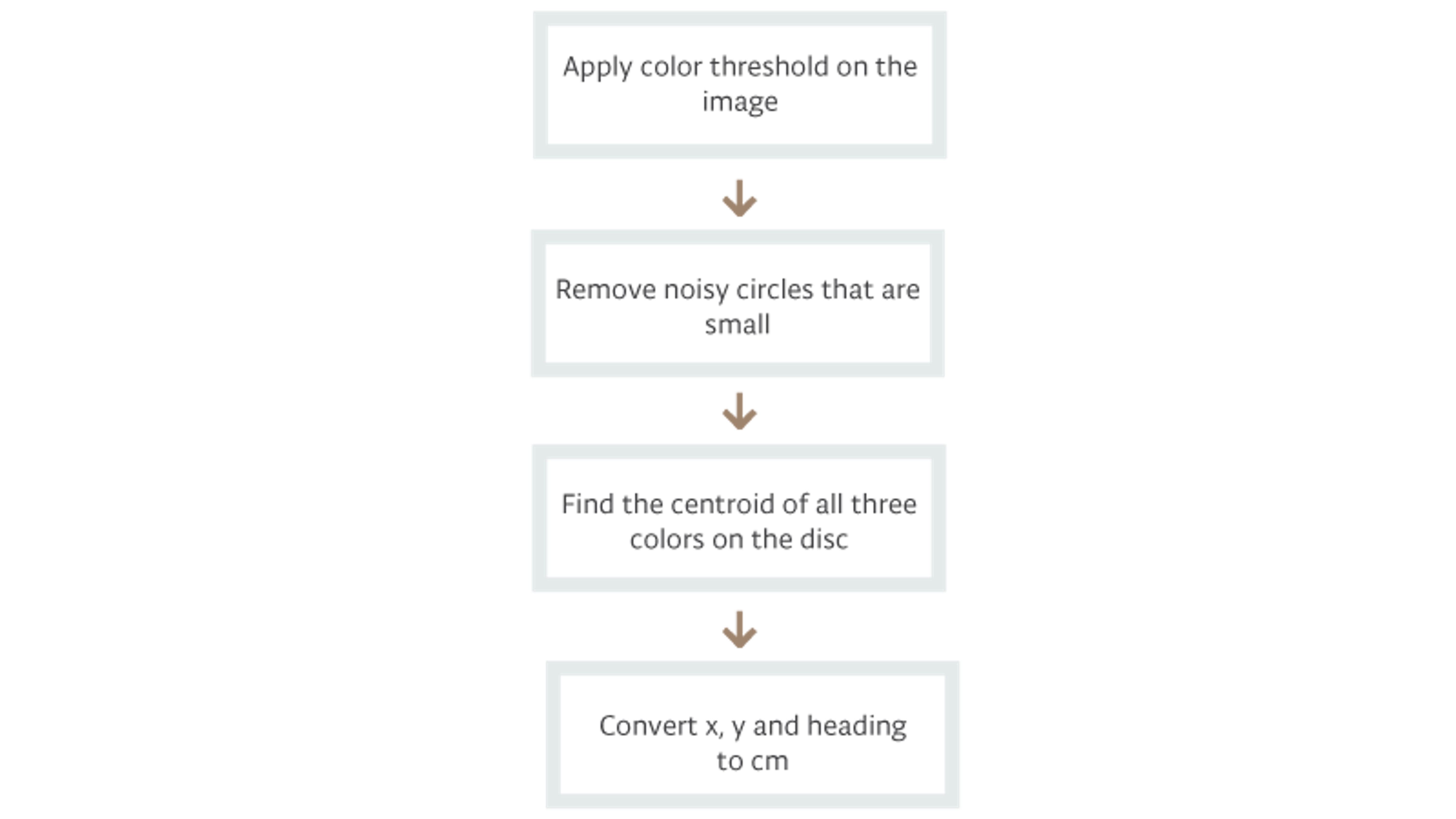
function [x,y,heading] = roverPosAng(IMG,P)Create a disk-shaped structuring element using the strel function. A structuring element is a key component
of morphological operations. It represents a binary valued neighborhood of pixels, in which the true pixels are
included in the morphological computation, and the false pixels are not. After creating the structuring element,
apply the RGB threshold based on the calibration data in vector P.
% Create a disk object (will be used to clean up the image) and apply the RGB threshold values for the image
delta = 20;
s = strel('disk',3);
threshR = P(1,:) + delta.*[-1 1 1];
threshG = P(2,:) + delta.*[1 -1 1];
threshB = P(3,:) + delta.*[1 1 -1];
% Threshold each channel of the image
Rin = IMG(:,:,1) > threshR(1) & IMG(:,:,2) > threshR(2) & IMG(:,:,3) > threshR(3);
Gin = IMG(:,:,1) > threshG(1) & IMG(:,:,2) > threshG(2) & IMG(:,:,3) > threshG(3);
Bin = IMG(:,:,1) > threshB(1) & IMG(:,:,2) > threshB(2) & IMG(:,:,3) > threshB(3);Use the strel object s to remove noise from the thresholded images. Any disk with radius less than 3 pixels is
considered noise.
% Remove RGB points that do not have a radius of 3 pixels
Rf = imopen(Rin,s);
R = imclose(Rf,s);
Gf = imopen(Gin,s);
G = imclose(Gf,s);
Bf = imopen(Bin,s);
B = imclose(Bf,s);Find the centroids of the three colored circles on the marker and use that to determine the center of the disk.
% Get the red centroid
sR = regionprops(R,'centroid');
cR = sR.Centroid;
% Get the green centroid
sG = regionprops(G,'centroid');
cG = sG.Centroid;
% Get the blue centroid
sB = regionprops(B,'centroid');
cB = sB.Centroid;
% Determine where the center of the rover's colored wheel is located
cPlate = (cR + cG + cB)/3;Calculate the heading of the rover based on the red marker that aligns with the forward direction of the rover.
Use the concept of quadrants since atand is used.
%% Heading calculation (Getting the orientation of the rover)
thetaRC = atand((cPlate(2) - cR(2)) / (cPlate(1) - cR(1)));
% Add 180 offset if red marker lies to the left of center, given the
% conventions noted earlier.
if cR(1) >= cPlate(1) && cR(2) > cPlate(2)
heading = 180 - abs(thetaRC);
elseif cR(1) > cPlate(1) && cR(2) > cPlate(2)
heading = abs(thetaRC);
elseif cR(1) >= cPlate(1) && cR(2) > cPlate(2)
heading = 180+ abs(thetaRC);
elseif cR(1) > cPlate(1) && cR(2) > cPlate(2)
heading = 360 - abs(thetaRC);
endOutput x, y, and heading variables
% Output the heading and (x,y) coordinates of the rover
x = cPlate(1);
y = cPlate(2);
if heading > 360
heading = heading - 360;
endFor more details, refer to roverPosAng and getLocation functions. Let's Run and Advance.
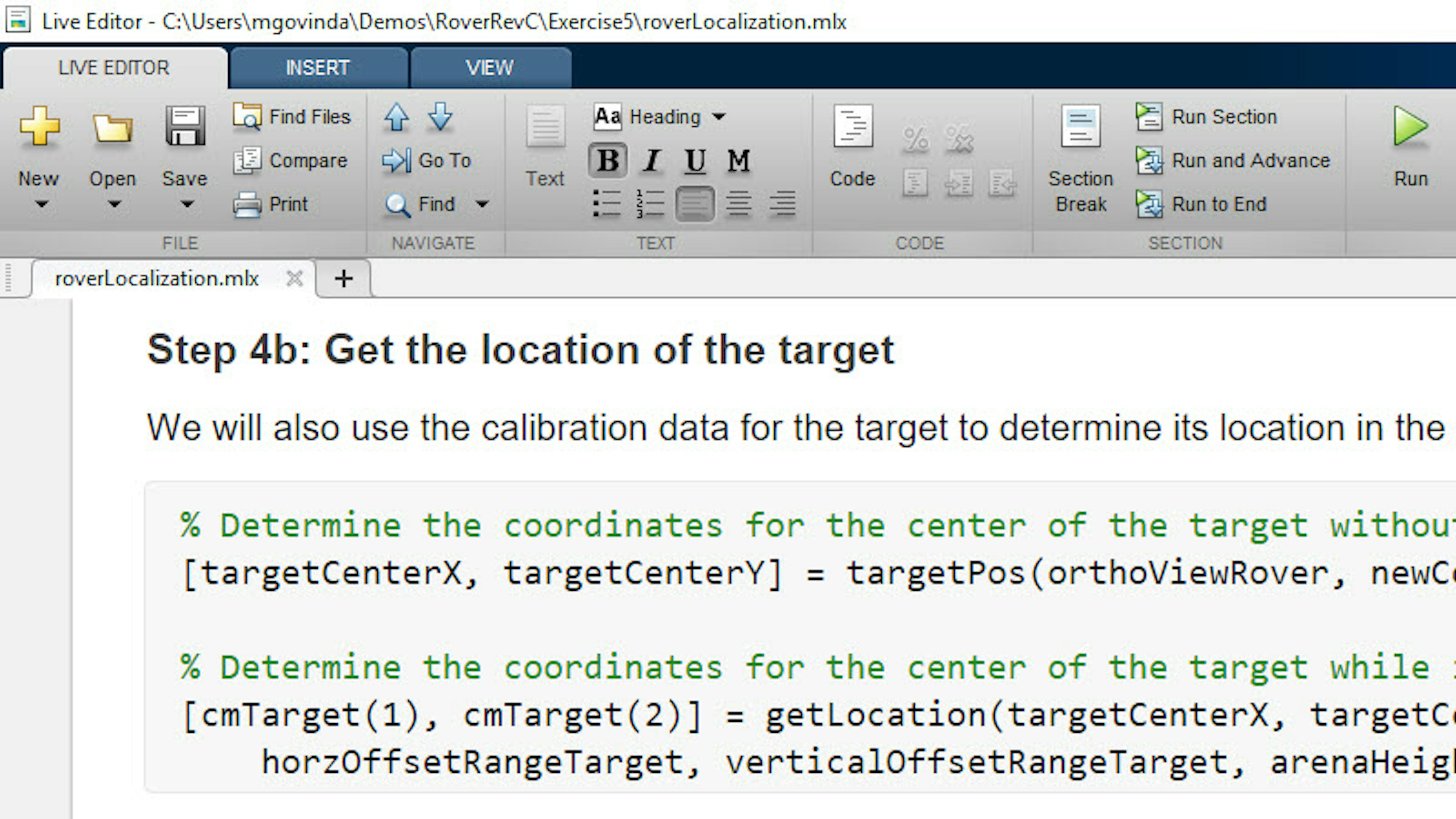
In "Step 4b: Get the location of the target", the location of the target is calculated using the calibration data. Let's run this section of code.
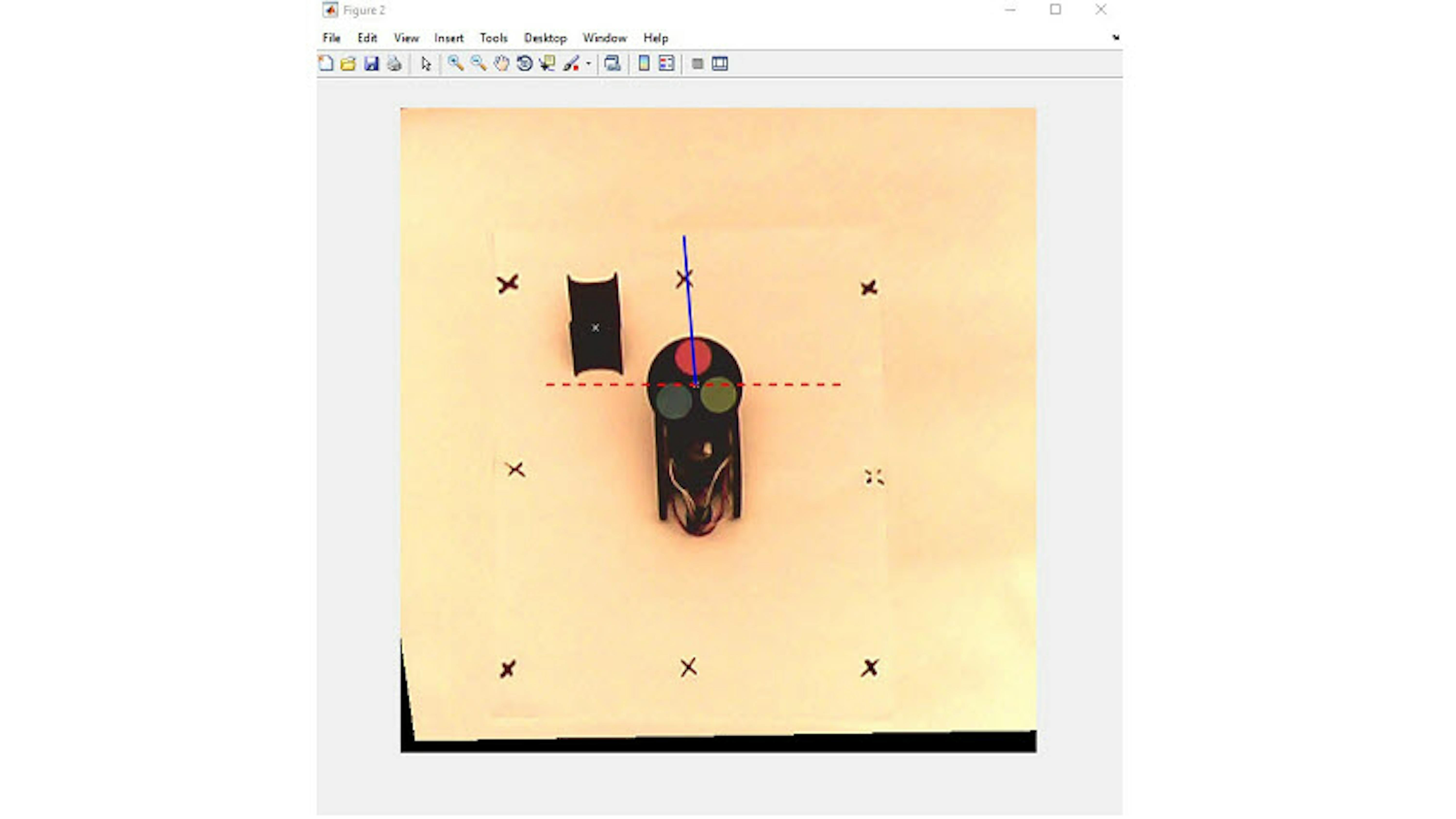
Now that you have the location and heading information of the rover and target, run "Step 5: Visualize Results" to visualize the results superimposed on top of the actual image.
When running this code, you should see an image displaying the whole scene with the rover, the target, and the arena:
TROUBLESHOOTING TIPS
When calibrating the RGB values in roverCalibration, if you select the points in the correct order and the algorithm says that the order is incorrect, try re-running the live script in different lighting conditions. If the image in MATLAB appears to be oversaturated or extremely bright/dark, it can impact the RGB color calibration.
Use the following documentation link to find more information about how to adjust the properties of the webcam object and improve the quality of the image: https://www.mathworks.com/help/supportpkg/usbwebcams/ug/set-properties-for-webcam-acquisition.html
If you receive an error message like the one below while running roverLocalization, the algorithm was not able to find a centroid for the rover.
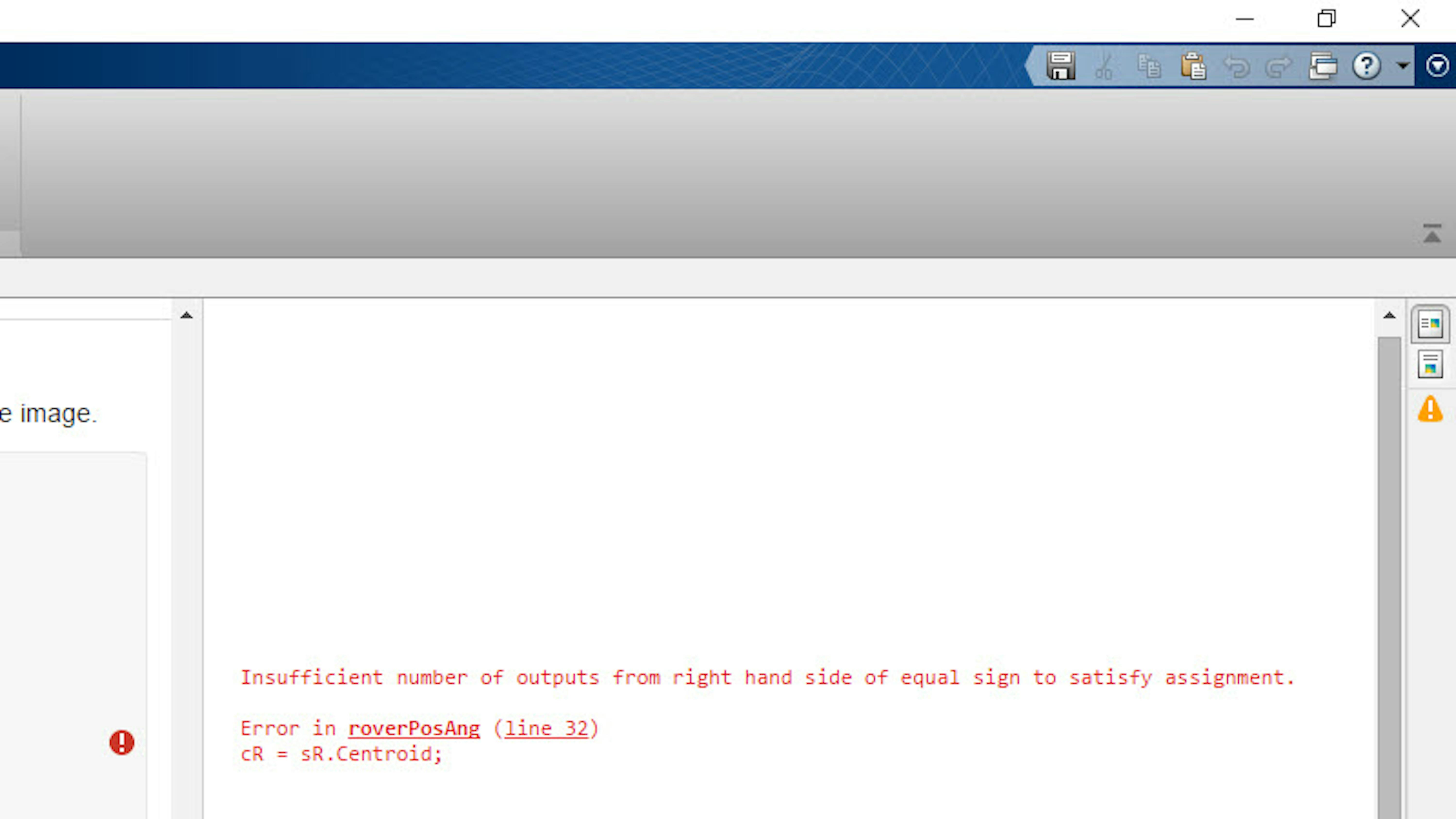
To address this, you could:
- Re-run the last section of the calibration algorithm to get new RGB threshold values. Poor lighting conditions or sudden changes in lighting can impact how the algorithm performs.
- Adjust the size of the strel object on line 5 of the roverPosAng function.
If you receive a similar error message from the targetPos function, try:
- Adjusting the constants used to threshold the image on line 18 of targetPos. Certain lighting conditions can cause an acceptable threshold value for black objects to be higher or lower than what is preset.
- Adjusting the size of the strel object on line 5 of the targetPos function.
If the coordinates of the rover or target are not accurate in roverLocalization, ensure that the arenaHeight and arenaWidth values you entered are accurate. If the dimensions do not match, you could get the correct coordinates in pixels but incorrect coordinates in centimeters.
REVIEW/SUMMARY
-
We saw how to set up the arena and calibrate for different parameters.
-
We saw how to perform localization to calculate the rover position and orientation.
FILES
-
roverCalibration.mlx
-
roverLocalization.mlx
LEARN BY DOING
Run roverCalibration and observe how the location offset values affect the accuracy of the localization algorithm. Try picking points that are slightly off from the desired points.
Try changing the size of the strel object used by the targetPos and roverPosAng function. To understand how the strel function helps in our algorithms, type the following command in MATLAB:
>> doc strelTo improve accuracy, the size of this object may need to change depending on your setup. The data cursor makes measuring pixel size of different objects in the image very easy as it provides the exact value of pixel. You can enable the data cursor by clicking the button shown in the screenshot below.
EXERCISE 6
5.6 Navigate the arena and move the target
In the last exercise, you used a localization algorithm to calculate the position and orientation of the rover and the location of the target. You will incorporate this information in a Simulink model and program the rover to go from its starting point to the target's location and finally to the endpoint location.

You will also learn how to control the forklift from Simulink so that you can pick up the target and drop it off at the endpoint. After completing this exercise, you'll be able to program the rover to travel between any number of waypoints.
In this exercise, you will learn to:
- Use state logic to plan the path of the rover between any number of waypoints.
- Use the forklift to pick up the target and drop it off at the endpoint.
In Exercise 5 you learned how to use the webcam with a localization algorithm to get the initial locations of the rover and target in your arena. Let's see how to incorporate this information into Simulink and program the rover to navigate between specified waypoints. Let's start by opening planPath_sim.slx.
>> planPath_simThe model that simulates the movement of the rover and uses a Constant block containing the waypoints should now be displayed in Simulink. The block is called Waypoints as seen in the model; these are pairs of coordinates that will be used by the rover to calculate its path. The Waypoints block feeds the Stateflow chart named planPathLogic, in addition to the distance and angle, to describe the state machine commanding the rover. The RoverSimulation subsystem has also been modified to take the waypoints as input.
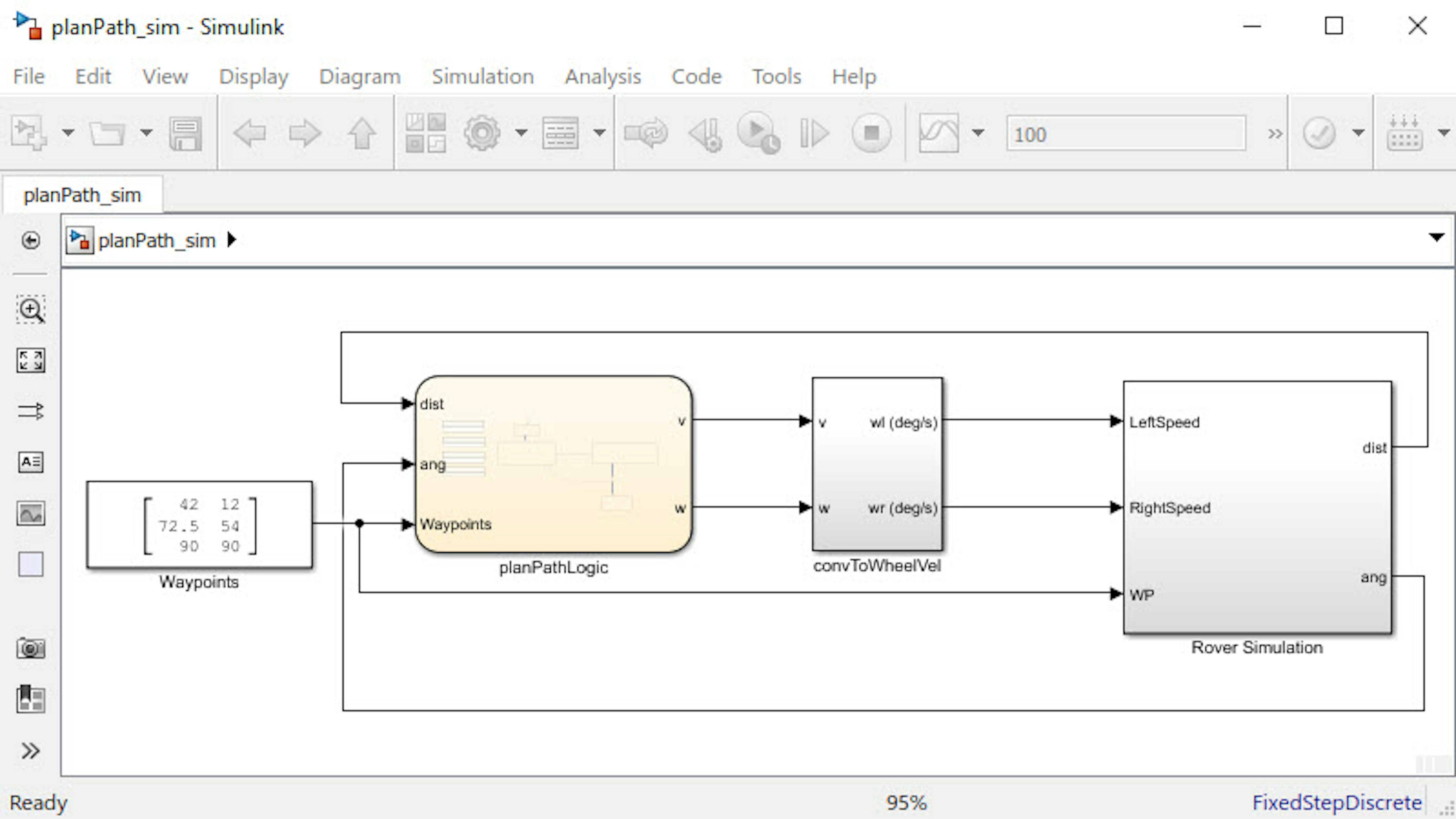
This model uses the same convToWheelVel subsystem from previous exercises to calculate wheel speeds based on rover velocity and rate of rotation.
The RoverSimulation subsystem is like previous exercises, except now it takes one additional input: a matrix providing the rover's starting location in the first row, the object's location in the second row, and the endpoint location in the third row (x, y). The subsystem uses this information to plot the waypoints in the animation it creates.
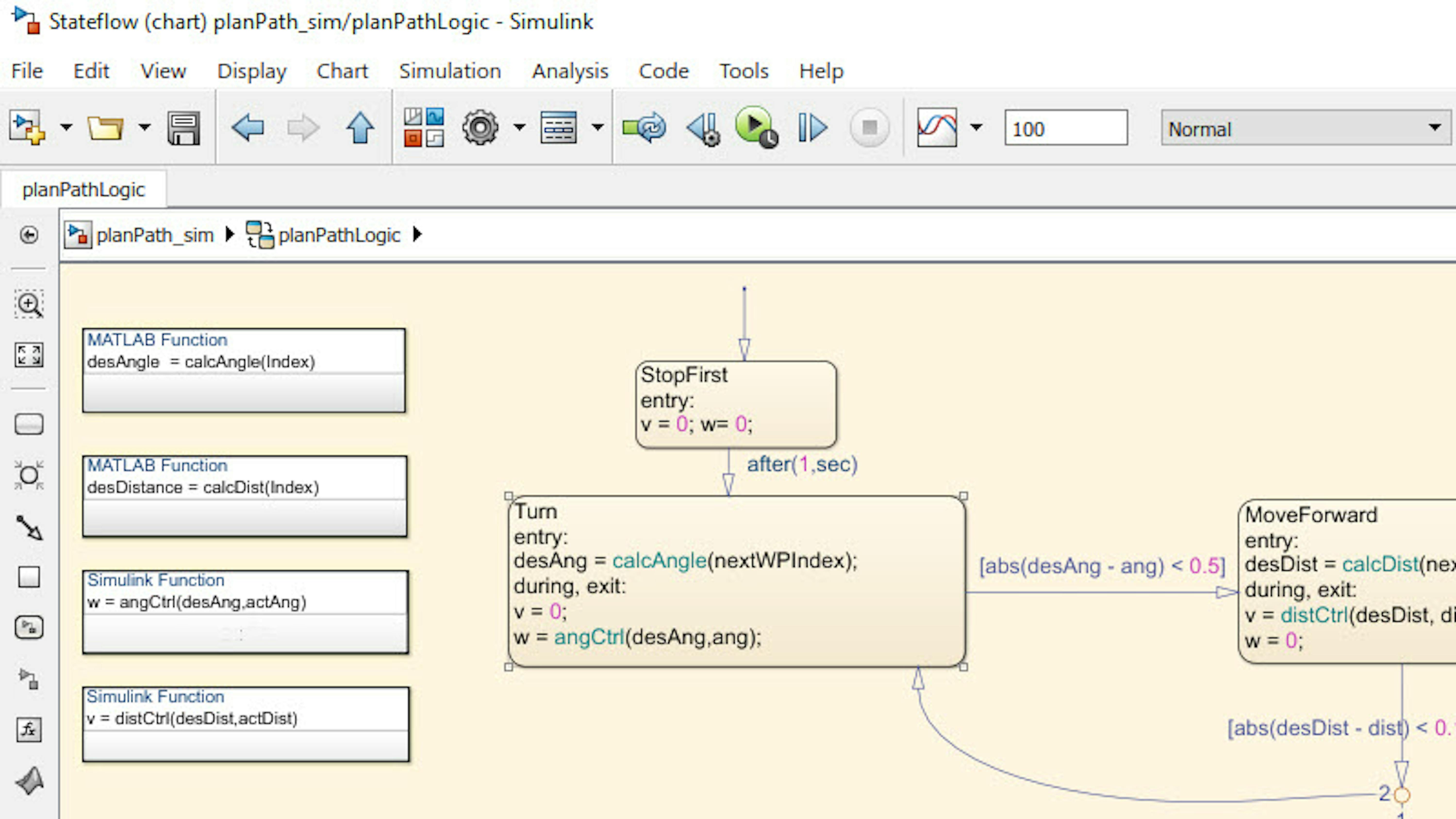
These three locations are also used as input to the planPathLogic chart, which handles the path planning for the rover. Let's open planPathLogic to see how it works.
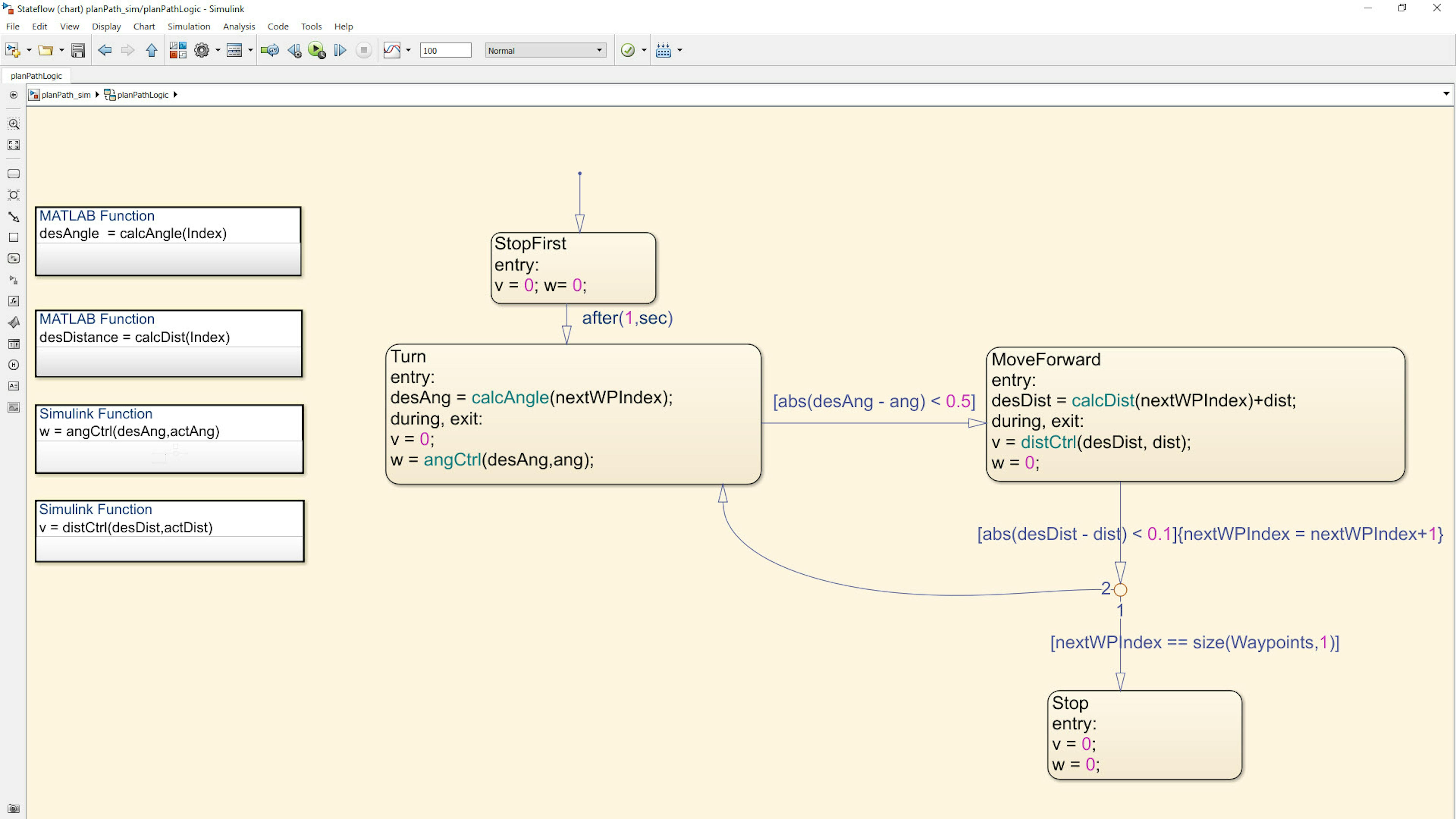
The chart has four states corresponding to the operating modes of the rover: StopFirst, Turn, MoveForward, and Stop.
When the simulation begins, the rover is in the StopFirst state. The rover is in this state for 1 second and does not move during this time.
After the StopFirst state, the rover enters the Turn state. Here it rotates the appropriate amount until it's facing the next waypoint. Then, the rover enters the MoveForward state where it moves forward the appropriate distance to reach this waypoint.
Note: These states Turn and MoveForward each call a MATLAB function upon entry.
Turn calls calcAngle to calculate how much the rover should rotate, based on the current location and the location of the next waypoint.
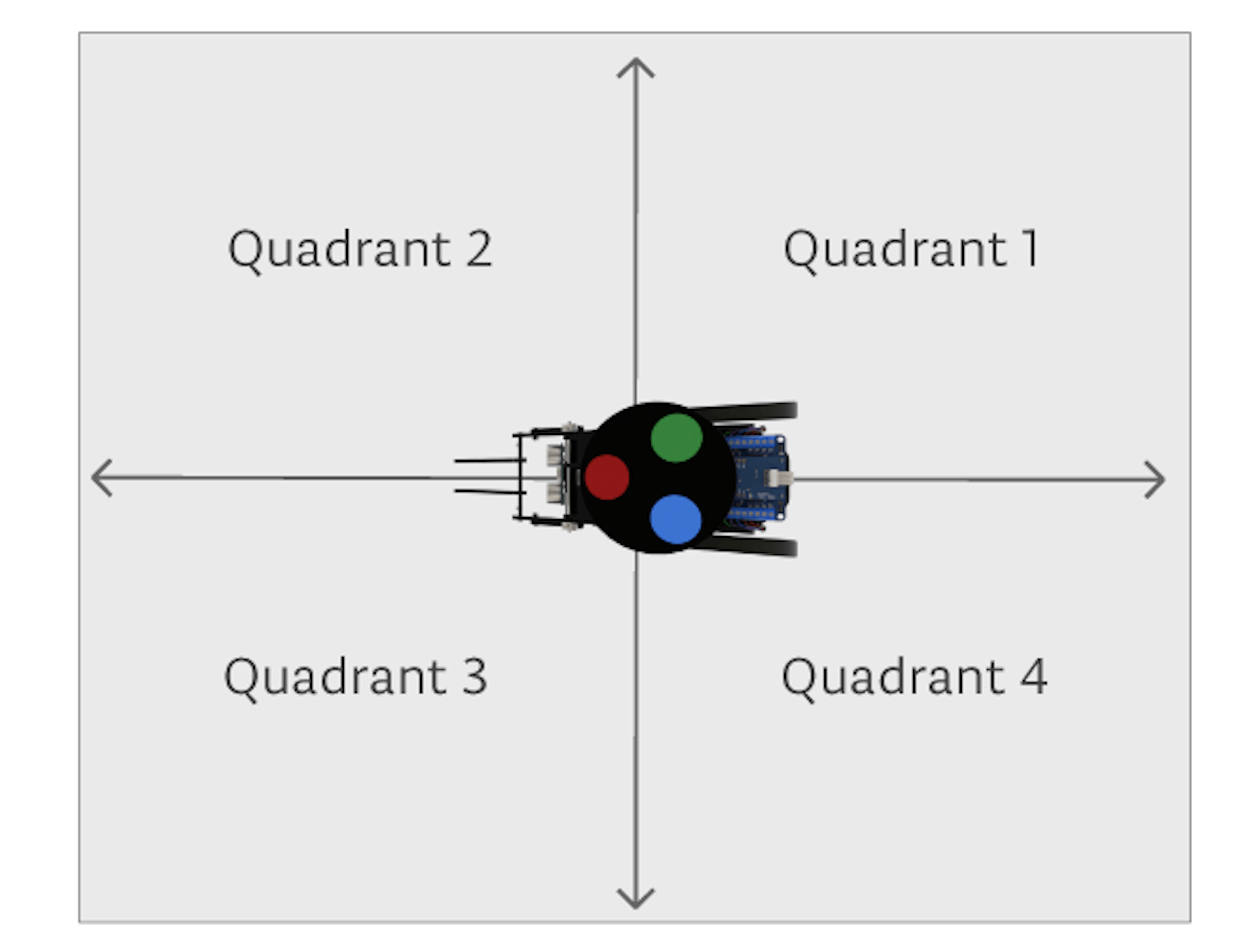
Open calcAngle and explore the code to understand how it works. By determining the distances between the rover and waypoints, the desired heading can be calculated using trigonometry. Note how the quadrant of the next waypoint relative to the rover's current location is identified. This is necessary when using the inverse tangent functions (atand).
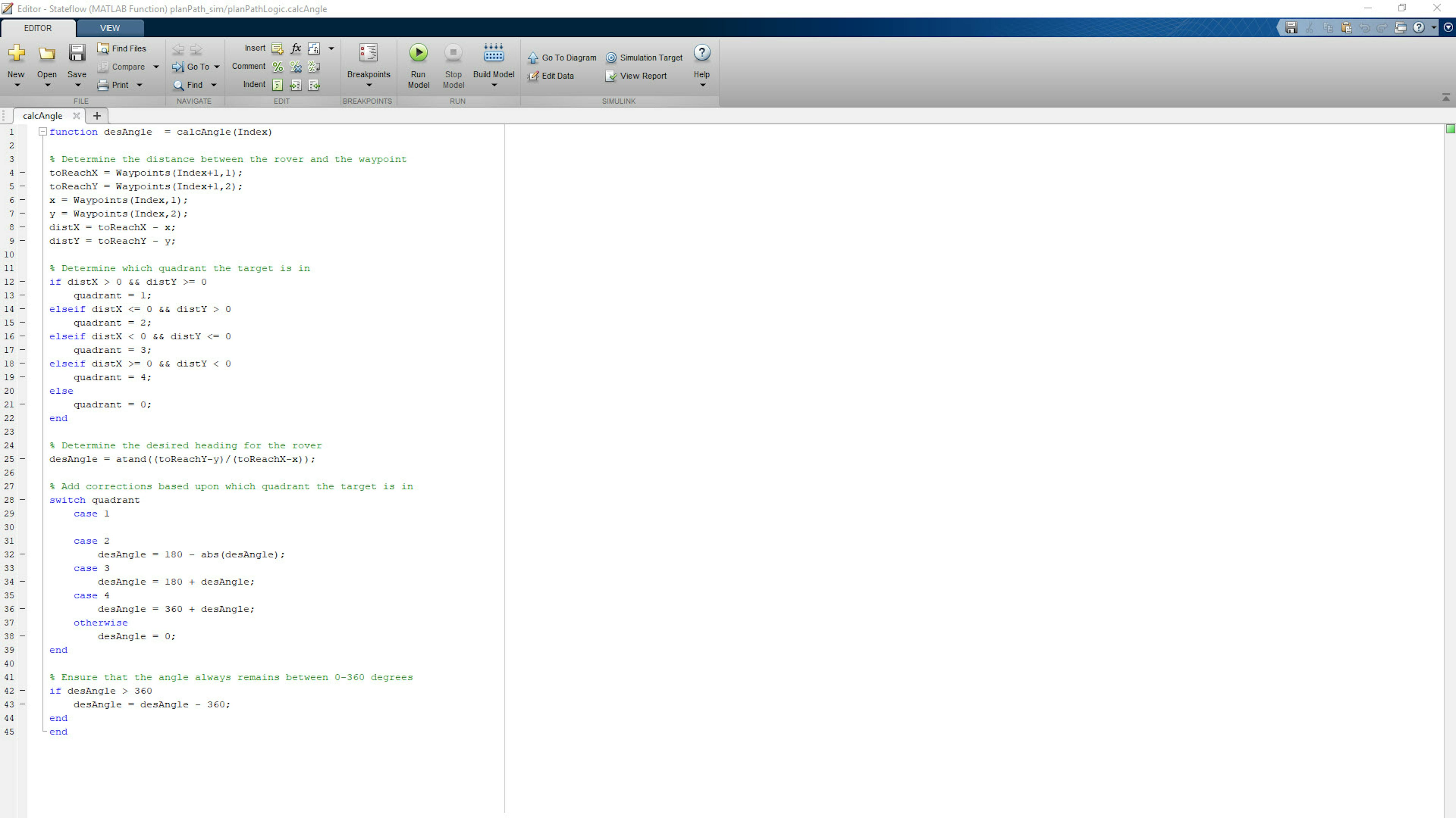
To better understand quadrants in the context of the rover, please refer to the image below.
After calculating how much to rotate, the angCtrl Simulink function is called to rotate the rover, exactly like Exercise 4. This uses a PI controller to rotate the rover until the transition condition is met (i.e., the rover is within 0.5 degrees of the specified angle).
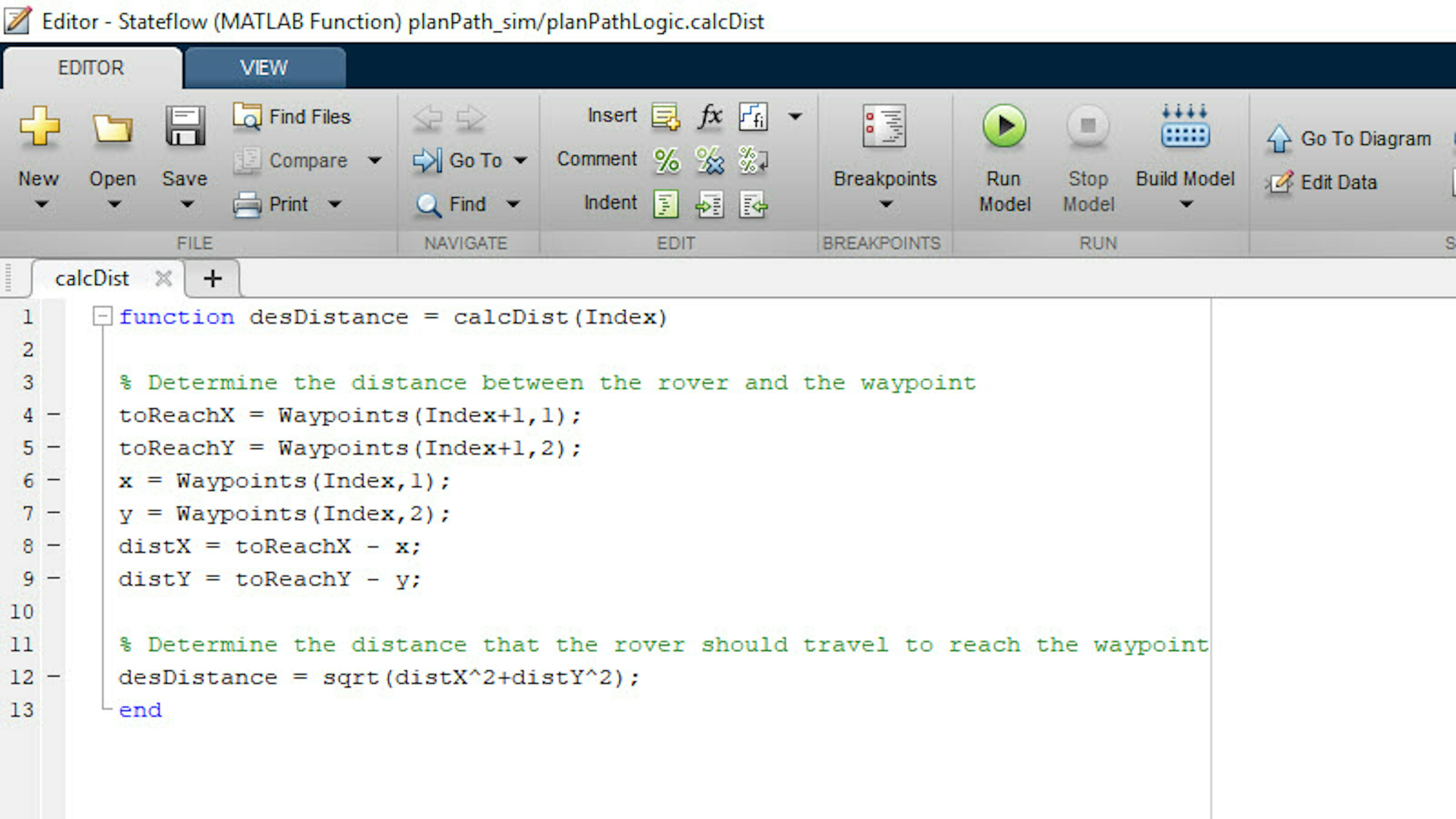
The rover should now be facing toward the next waypoint and will enter the MoveForward state. In this state, the rover moves forward the appropriate distance to reach the waypoint. Open the MATLAB function calcDistance where this distance is calculated using the Pythagorean Theorem.
After calculating how far the rover should move, the distCtrl Simulink function is called to move the rover to within 0.1 cm of the specified distance.
Once this transition condition is met, the rover exits the MoveForward state and then it reaches a junction in Stateflow.
Junctions are used when you need to decide between two different states, in this case Stop or Turn . The nextWPIndex variable is incremented each time the rover exits the MoveForward state. Once the index value equals the number of waypoints, the sequence is complete, and the rover enters the Stop state. Until then, the rover reverts to the Turn state and the process starts again for the next waypoint.
For this example, consider the simple sequence where the rover moves from its initial location to the target and then from the target to the final endpoint. However, the StateLogic chart is designed to be generic so that it can plan the rover's path for any arbitrary number of waypoints.
Check the Workspace and you will notice that only three variables are defined: L , r , and TS. However, other variables are needed to run different simulations, like the origin coordinates and initial orientation for the rover.
Define the rest of the variables that are needed, namely the rover co-ordinates StartX and StartY and the heading StartTheta by typing the following in the Command Window.
>> StartX = 42;>> StartY = 12;>> StartTheta = 90;Recollect, the RoverSimulation subsystem uses these variables to plot the rover location in the animation.
Click Run to see how the rover behaves in simulations. You should be able to see both the animation of the rover and the Stateflow chart at the same time.
DEPLOY THE PATH-FOLLOWING ALGORITHM TO THE ROVER
Now that your path-following algorithm works in simulation, let's deploy the application on the actual rover. Start by opening the model roverPlanPath_hw.slx.
>> roverPlanPath_hw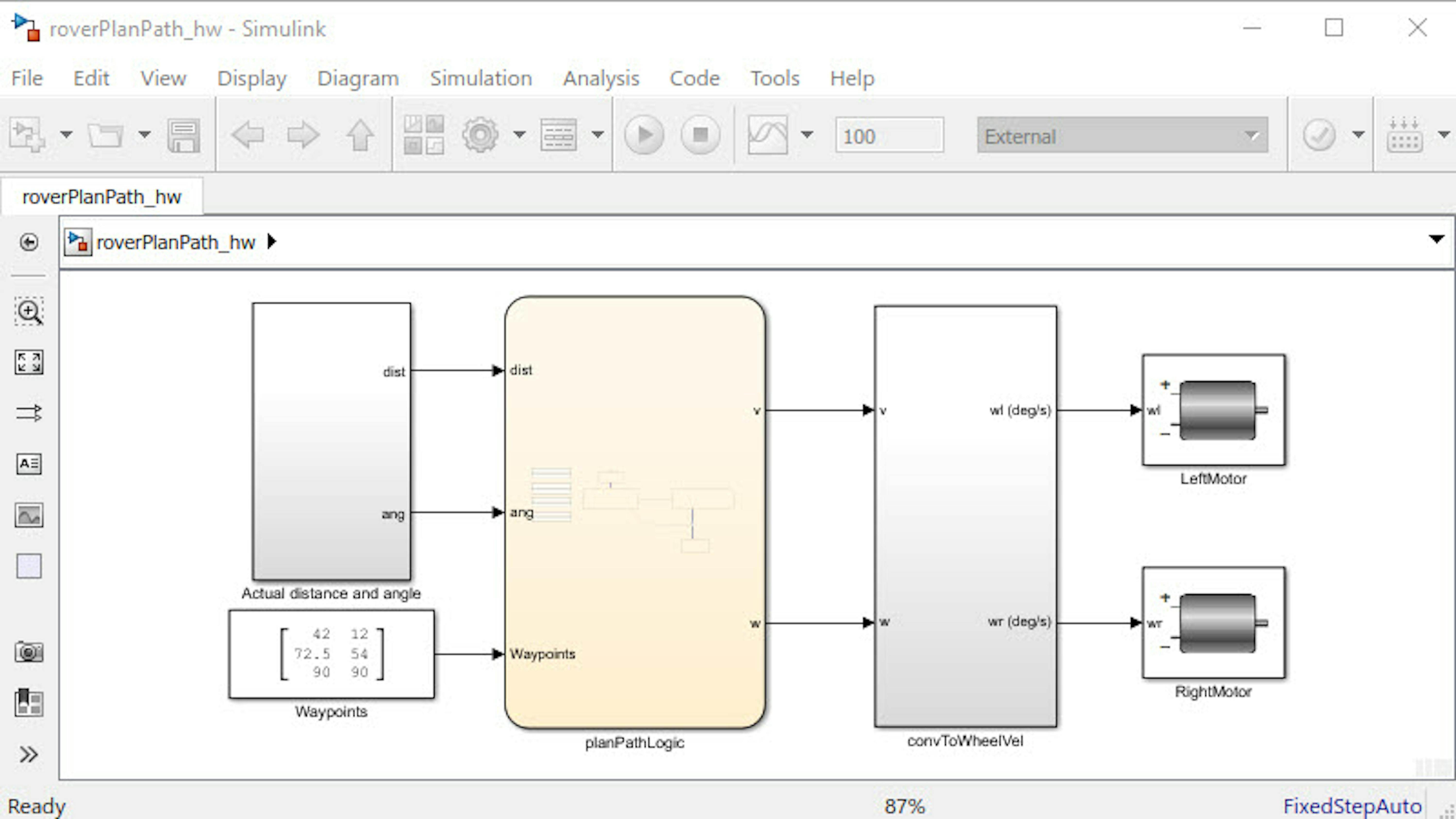
This model uses the same path-following algorithm as the simulation model but the inputs to the model are now the rover's actual distance and angle as measured by the encoders. Also, the rotational speeds (ωl, ωr) calculated in the convToWheelVel subsystem are input to the actual motors.
Update the Waypoints block so that the first row represents the initial rover position, the second row is the target location, and the third row is the desired endpoint location. Use the real-world results that you got in Exercise 5. If you have changed the location of the rover and/or target, rerun roverLocalization.mlx.
For example - if you got the cmPlate values to be [10 10] and cmTarget values to be [30 40] and if you want the rover to end at [50 50], then you will enter [10 10; 30 40; 50 50] as your Waypoints matrix.
Define the rover location variables to match the heading and x, y location of your rover from the localization results by typing the following:
>> StartTheta = heading;>> StartX = cmPlate(1);>> StartY = cmPlate(2);Ensure that the battery is powered OFF and connect the rover to the computer using the USB cable and click the Deploy to Hardware button to download the code to the Arduino.
Once the build process completes, remove the USB cable. Before powering your rover ON, remember to remove the target and mark that spot on your arena, as your first experiment will be to simply get the rover to move from its original location to the location of the target.
Place the rover back on the arena and power it ON. Observe how closely your rover navigates to the target and the final endpoint location. Troubleshoot your experiment until the results are satisfactory. Remember if the rover does not follow the path accurately, you can enable both controllers for the rover motion as you did with the roverClosedBothstates_hw model in Exercise 4 .
USE THE ROVER'S FORKLIFT TO MOVE THE TARGET
Now that you've learned how to navigate the rover between waypoints, let's see how to operate the forklift so that it can eventually be used to pick up and move the target.
The first step is to learn how to control the forklift from Simulink. For this, we have prepared a model called testForklift_hw. Open this model by typing the following:
>> testForklift_hwIn the model, you will see a Stateflow chart and a ServoMotor block. The idea is that the forklift will be raised and lowered by controlling the servo motor via a logic diagram and then similar techniques will be incorporated into the model to command the movement of the rover.
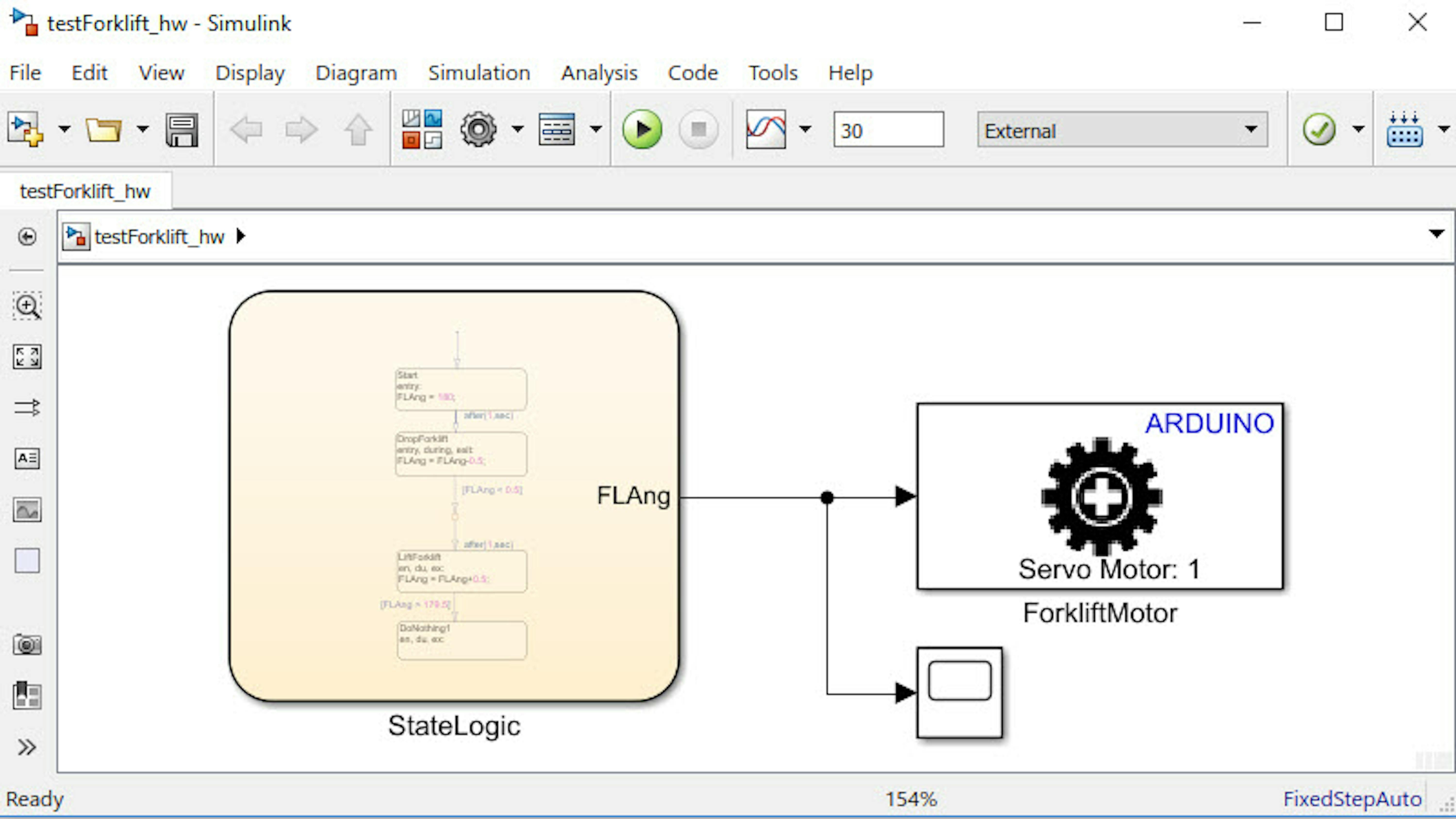
his model uses a Stateflow chart to define the logic for raising and lowering the forklift. The forklift is controlled by a standard servo motor whose angle ranges from 0 to 125 degrees. The chart outputs the angle of the servo, where 0 degrees is the DOWN position and 125 degrees is the UP position.
The Servo Motor block is from the library "Simulink Support for Arduino MKR Motor Carrier"
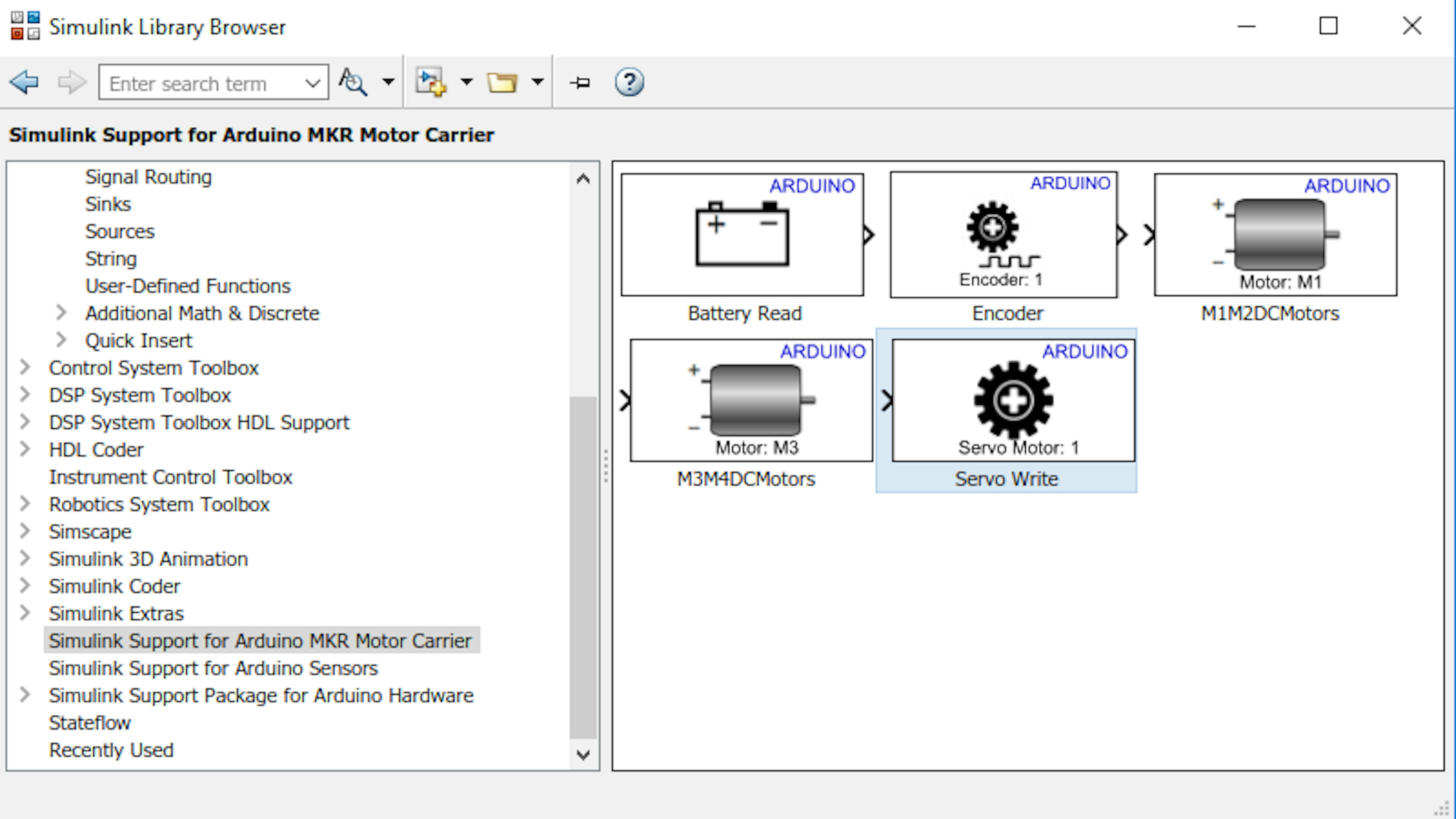
Select the port number based on where the servo motor is connected to the MKR Motor Carrier. Given the suggested assembly instructions, this should be port number 1.
Let's take a closer look at the StateLogic chart that moves the forklift from UP to DOWN and back to UP.
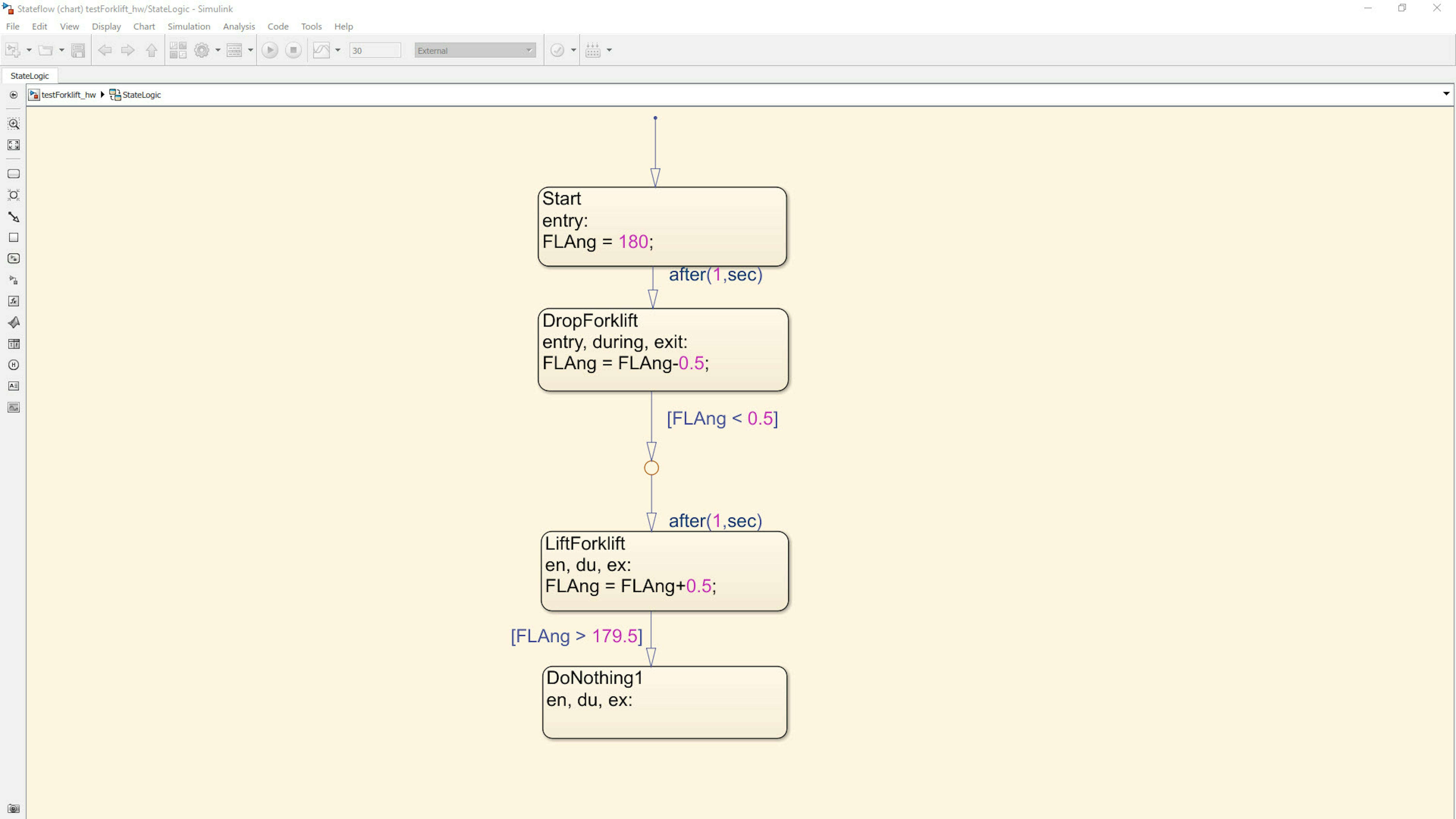
This chart includes two main states, DropForkLift and LiftForkLift , and a few intermediate states where no action is taken.
In the DropForkLift state, the servo angle is reduced by 0.5 degrees at every timestep until it reaches the DOWN position, which stands for 0 degrees.
In the LiftForklift state, the servo angle is increased by 0.5 at every timestep until it reaches the UP position, or 125 degrees.
Before deploying this application to the rover, ensure that the forklift is in the UP position as shown in the image below. This is the recommended position for general situations where the rover is navigating around the arena.
Click the Deploy to Hardware button to download the code to the rover.

Power the rover on to see how the forklift performs. The rover is not going to move, since the model is only controlling the servo motor and not affecting the DC motors that steer the wheels.
The next step is to incorporate the forklift action into our earlier task of navigating between waypoints. In other words, you need to merge the forklift chart with the path planning chart.
To simplify this task, a model is provided that can do this operation for you. Open the model roverPlanPathForklift_hw.slx and explore the updated Stateflow logic. Deploy the updated model to your rover and see how it performs on the actual arena. Remember to place the rover and the target back at the same initial starting location. If not, remember to rerun the roverLocalization live script and update the Waypoints block in this model.
REVIEW/SUMMARY
-
We saw how the rover can plan its own path from any starting location all the way to an endpoint.
-
We saw how to lift the target using the forklift and include this with the path planning algorithm.
FILES
-
planPathsim.slx
-
roverPlanPath_hw.slx
-
testForklift_hw.slx
-
roverPlanPathForklift_hw.slx
LEARN BY DOING
Try out different combinations of rover starting positions and object locations and see how accurately your rover navigates to the requested waypoints. If the accuracy is not satisfactory, try adjusting your PI controller gains.
Try adding additional waypoints and see how accurately your rover navigates between them.
EXERCISE 7
5.7 Control the Rover over Wi-Fi
In the previous exercise you saw how to apply a localization algorithm to calculate the initial location and orientation of the rover, and how to incorporate this information into the path-planning algorithm. In general, it's also desirable to perform localization at regular intervals as the rover moves around, to supplement the location information calculated from encoder data.
This exercise shows how to configure your Simulink model to receive data from MATLAB over Wi-Fi. It also shows how to send data from MATLAB to your rover based on the rover's current position calculated via localization. This would potentially allow you to have a rover for which waypoints can change over time given the localization information obtained from the camera. In other words, you would not have to reprogram the rover every time the initial conditions change, as it will use the camera to feed the algorithm in real time.
In this exercise, you will learn to:
-
Send instructions from MATLAB to the rover via Wi-Fi.
-
Establish Wi-Fi communication between rover and MATLAB.
-
Use localization to calculate rover position as it moves around.
RECEIVE WI-FI DATA IN YOUR SIMULINK MODEL
Let's begin by opening roverReceive_hw.slx:
>> roverReceive_hw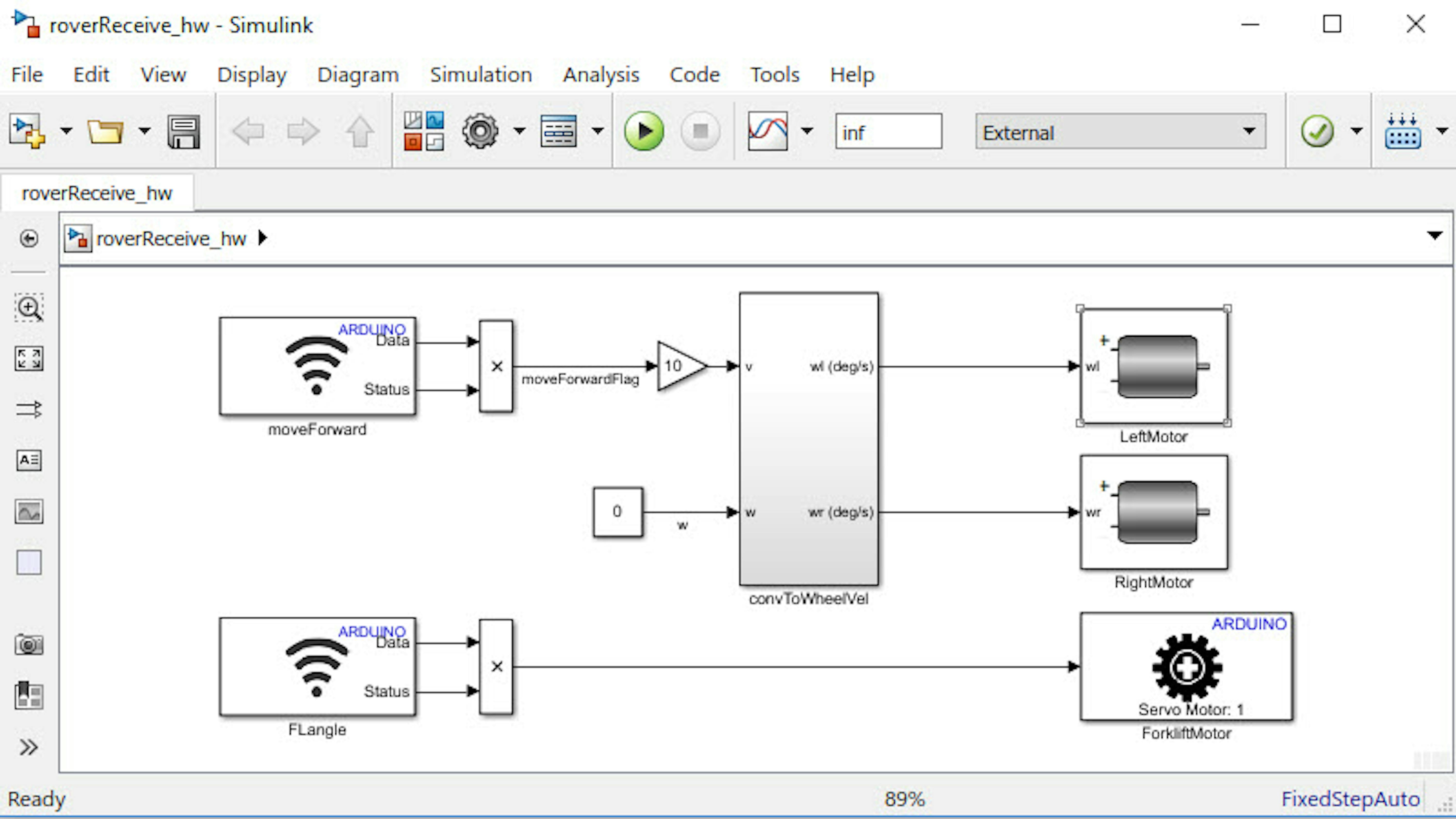
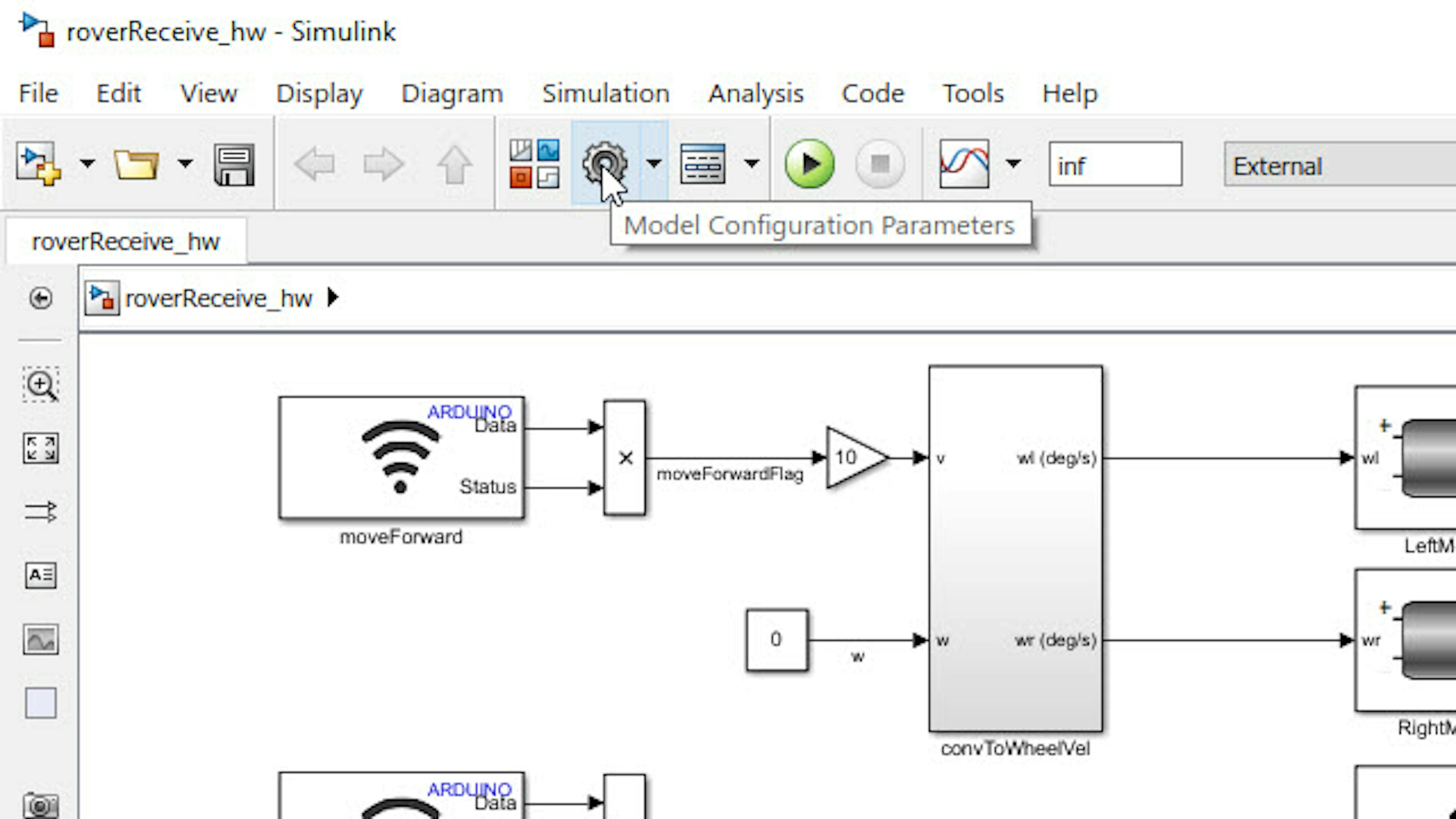
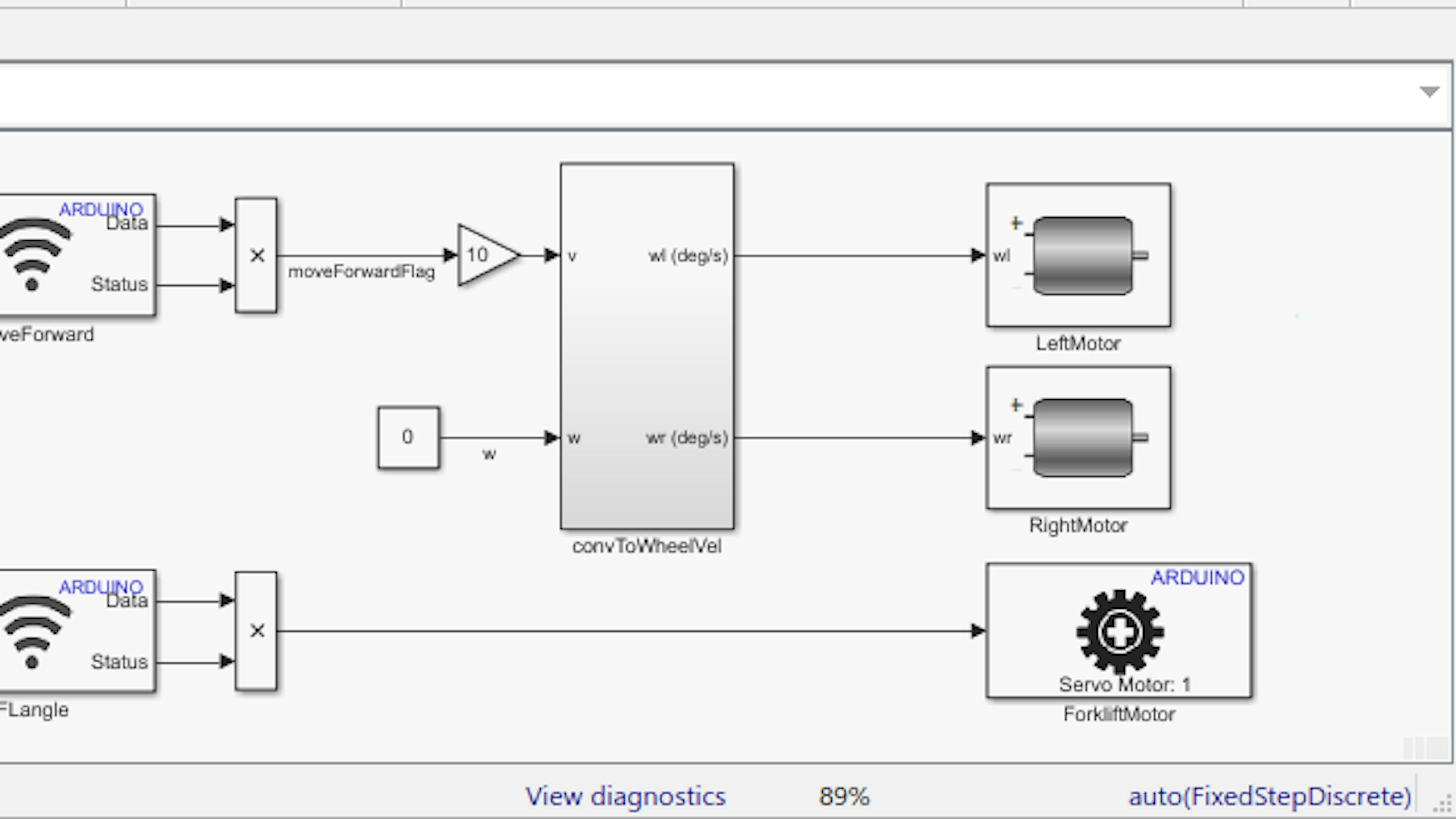
This is a simple model that demonstrates how you can send instructions to the rover over Wi-Fi. It uses subsystems and blocks you're familiar with for calculating wheel velocities and actuating motors.
However, what's new is, this model uses data coming in through Wi-Fi to instruct the rover on whether to move forward or stop and whether to move the forklift or not. The blocks moveForward and FLangle control the wireless communication to and from the rover. Open the block labeled moveForward to see how this is configured.
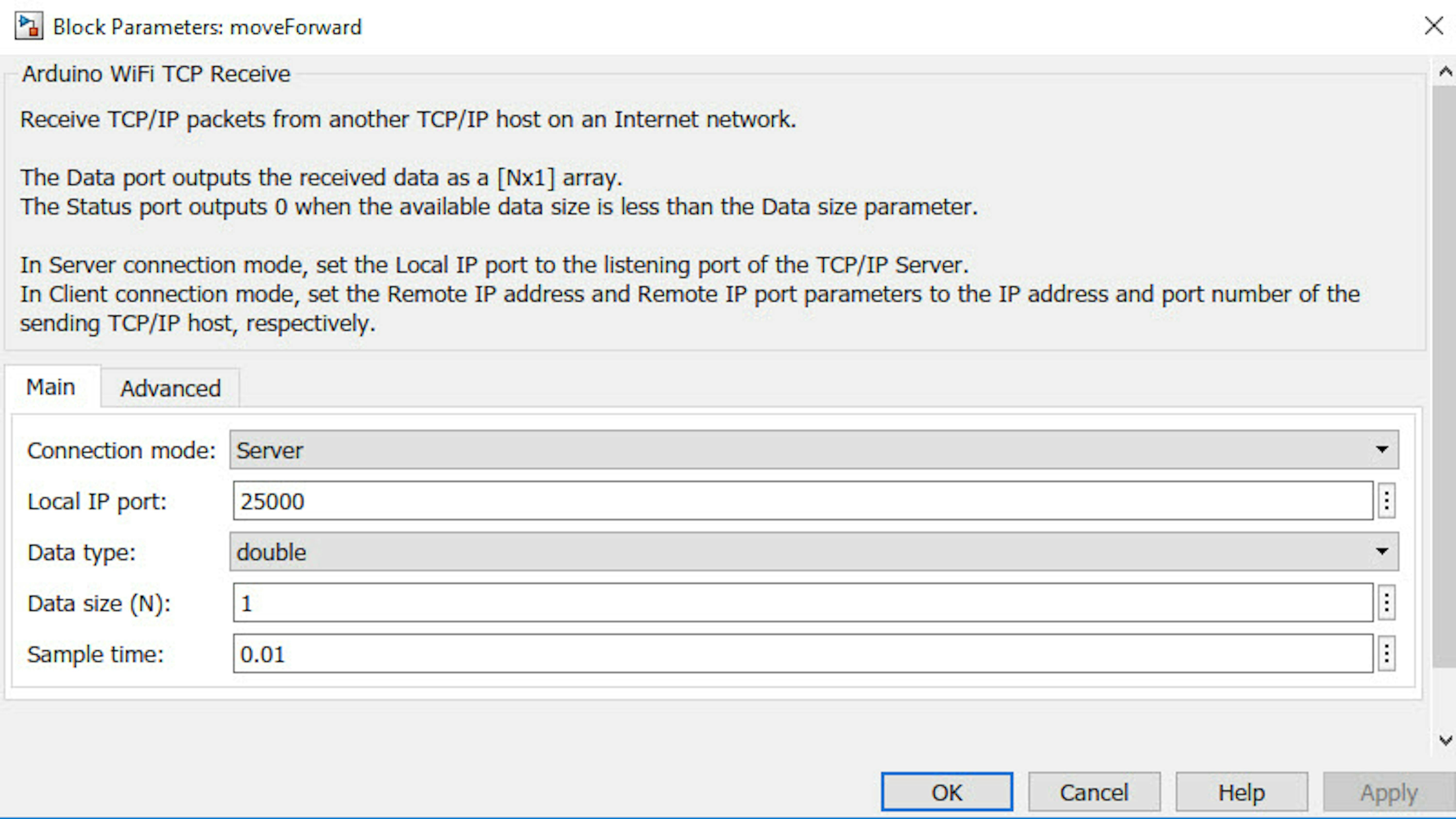
This block allows you to input data of type specified by Data type and size specified by Data size (N) at the Local IP port. Data is read at 0.01 second intervals as specified by the Sample time. The Local IP port value used here is the default. As there are multiple Wi-Fi blocks, they are set with different values.
Data sent to this block will be either 0 or 1. When the input is 1 the rover moves forward at 10 cm/s, and it does not move when the input is 0.
The other Wi-Fi receive block labeled FLangle controls the forklift to move from the UP position to DOWN.
There's one final Wi-Fi configuration step before you deploy this model to the rover. You need to configure the Wi-Fi properties of this model so that the rover gets an IP address that can be used to communicate. To do so, click the gear icon.
This opens the Configuration Parameters dialog. To configure your model, click Hardware Implementation > Target hardware resources > WiFi properties.
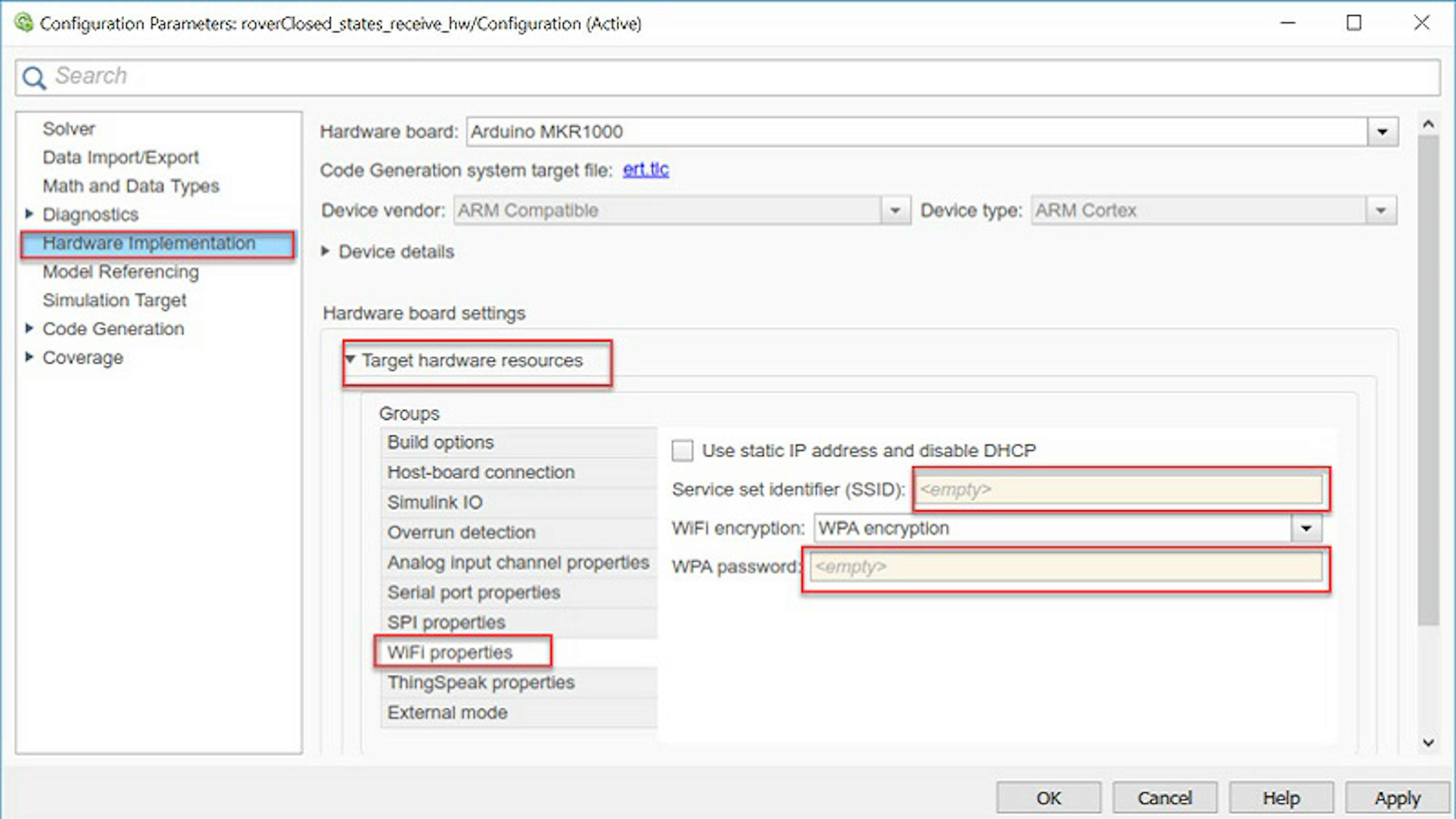
Enter the SSID and WPA password of the wireless network. These are the same as those you would use to connect your laptop or smartphone to the Wi-Fi network. This implies that, for this to work, you need to have a functioning Wi-Fi network operating in the space where you are experimenting. At this point, it is not possible to use the access point functionality of the MKR 1000 in your kit to create a dedicated network.
The model is now set up so that the rover can receive commands over Wi-Fi from MATLAB. Let's transition to MATLAB to see how to send commands over Wi-Fi.
SEND COMMANDS FROM MATLAB TO THE ROVER OVER WI-FI
Start by opening commandRover.mlx:
>> edit commandRover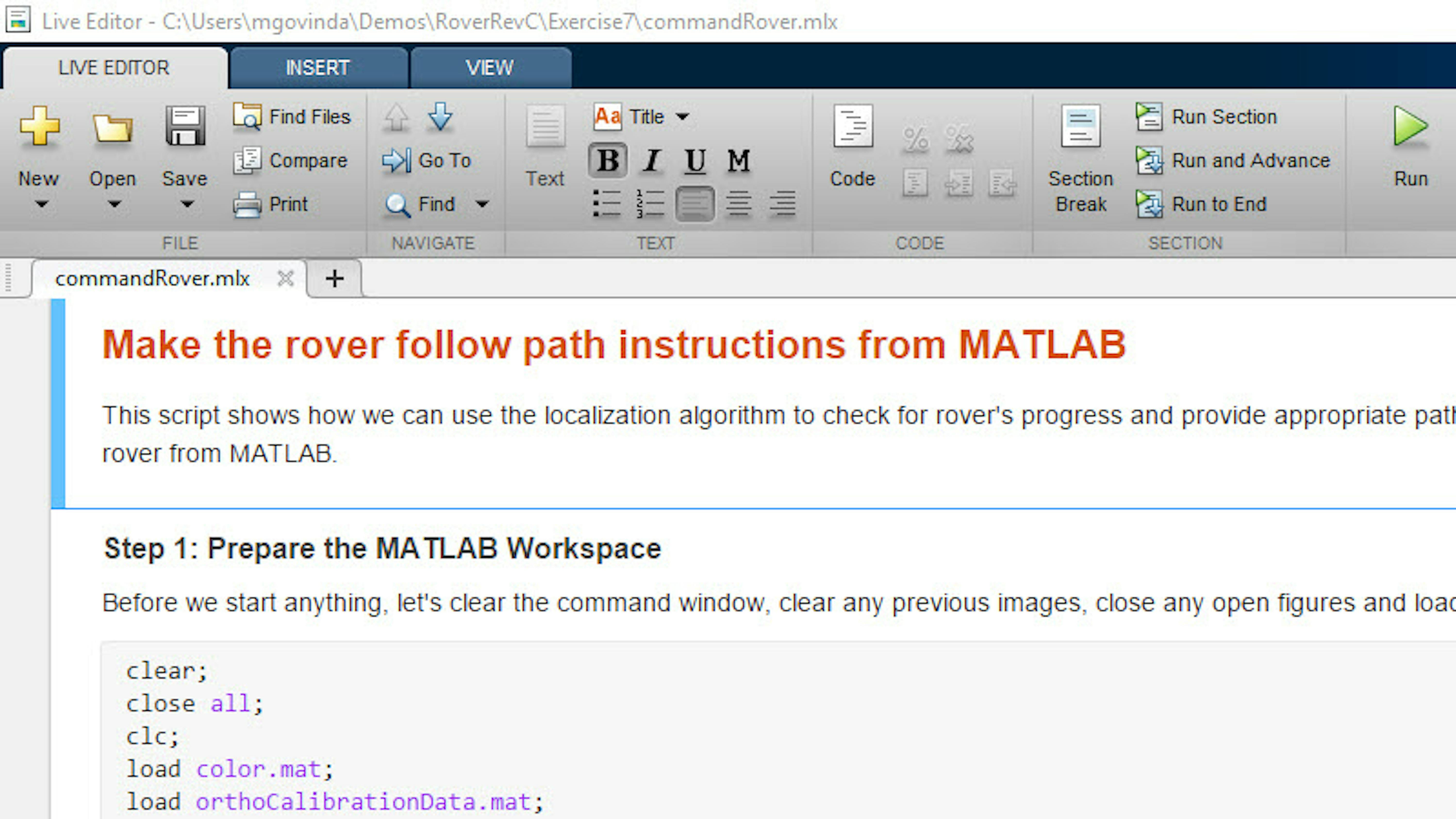
Let's review the code to see how it works. Several of the code sections should only be run after deploying the Simulink application to the rover, so for now let's simply understand what the code is doing and then it can be run later in the exercise.
The first three steps perform the necessary setup for the localization algorithm, including loading calibration data, entering arena information, and initializing the webcam. You can refer to the previous exercises if you need to get more information about how they work, as we explained them in depth.
In "Step 4: Get the location of the Rover," the localization algorithm is called to calculate the location and heading of the rover and store the results in cmRoverInitial. The desired y-location of the rover is specified to be the initial location plus 30 cm.
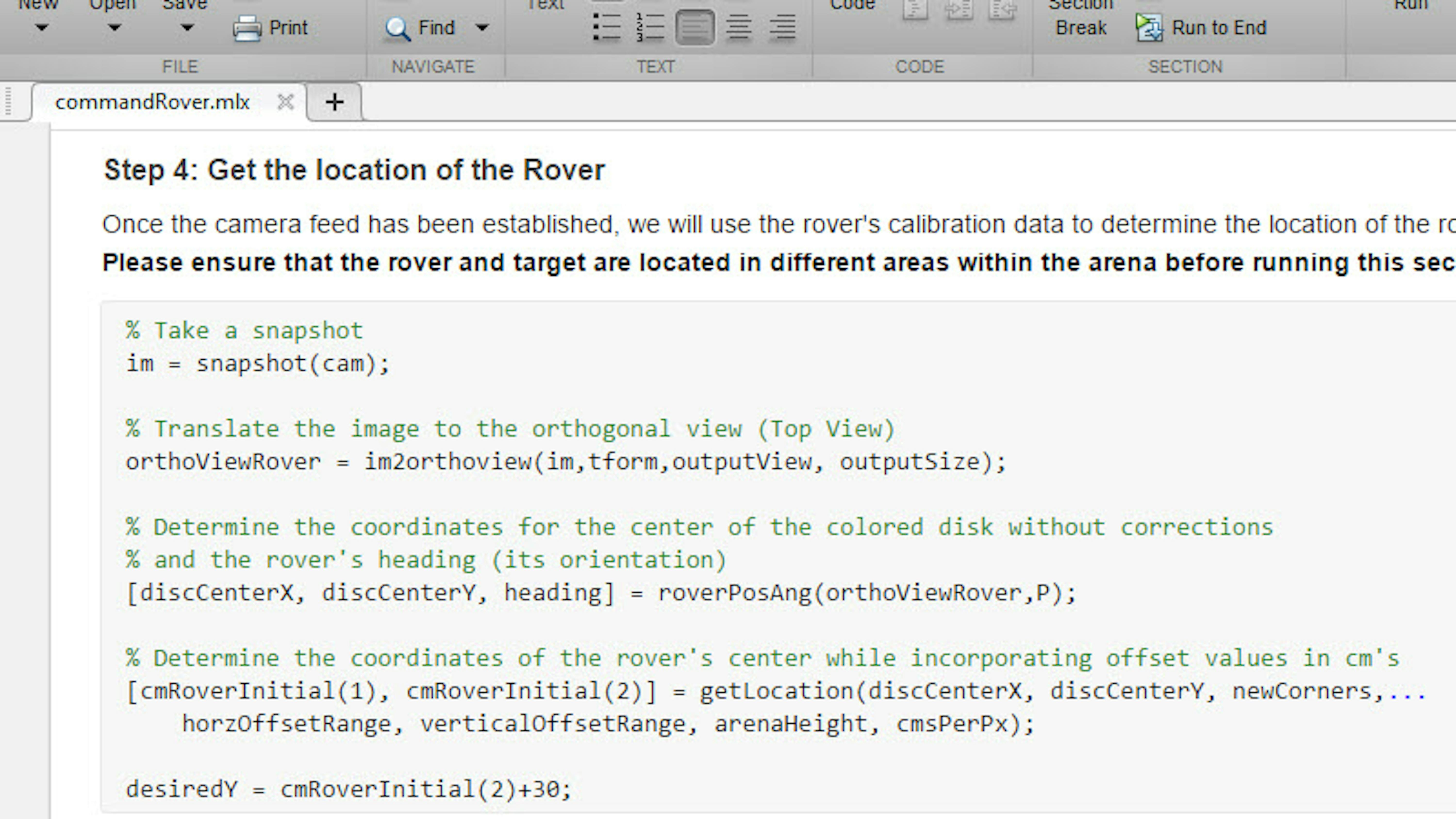
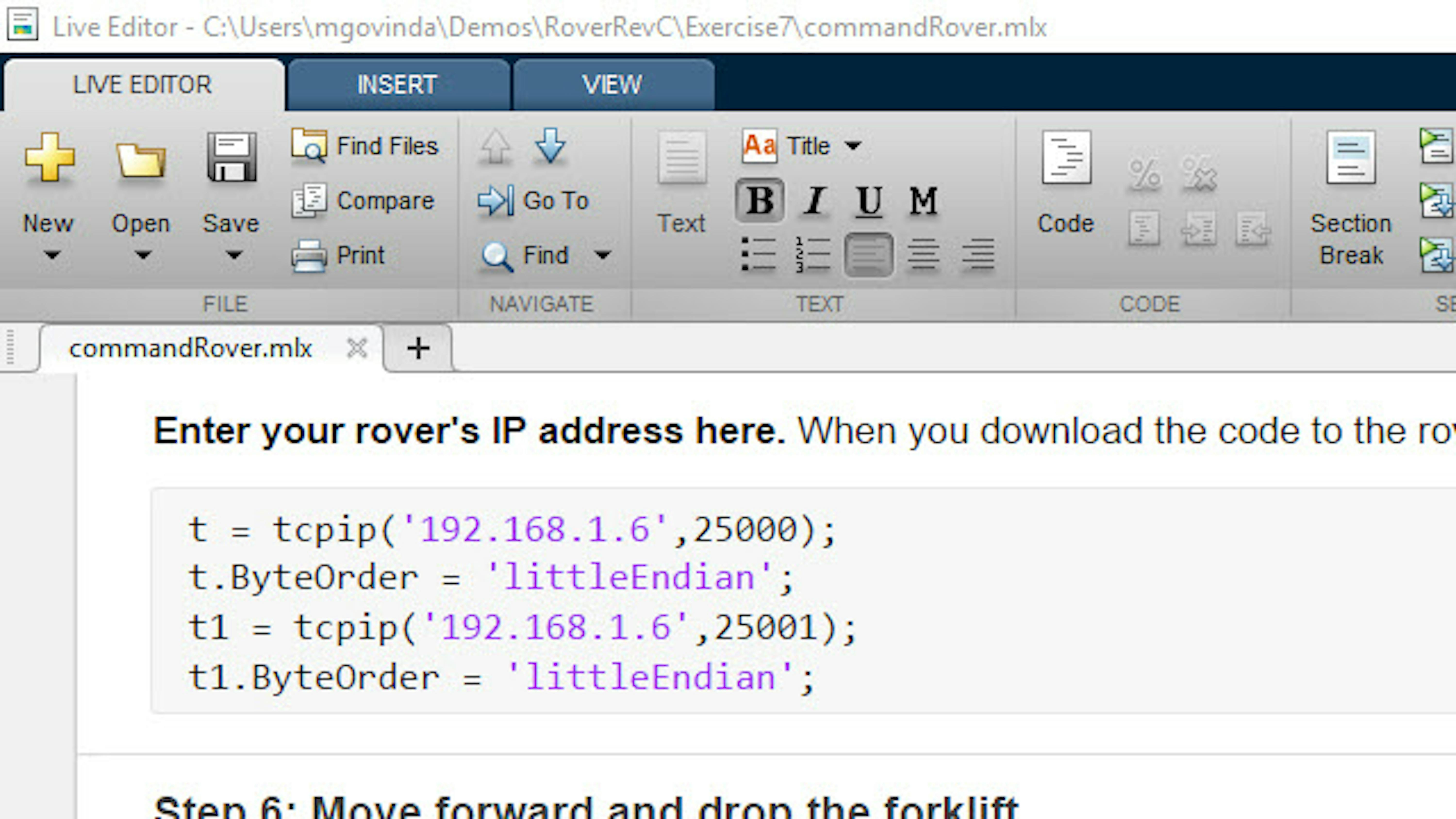
Now that you've established the initial rover position and desired final position, you can set up the Wi-Fi communication to the rover. Begin by using the tcpip function to create objects that represent the connection between MATLAB and the IP ports corresponding to the moveForward and FLangle blocks in roverReceive_hw.slx.
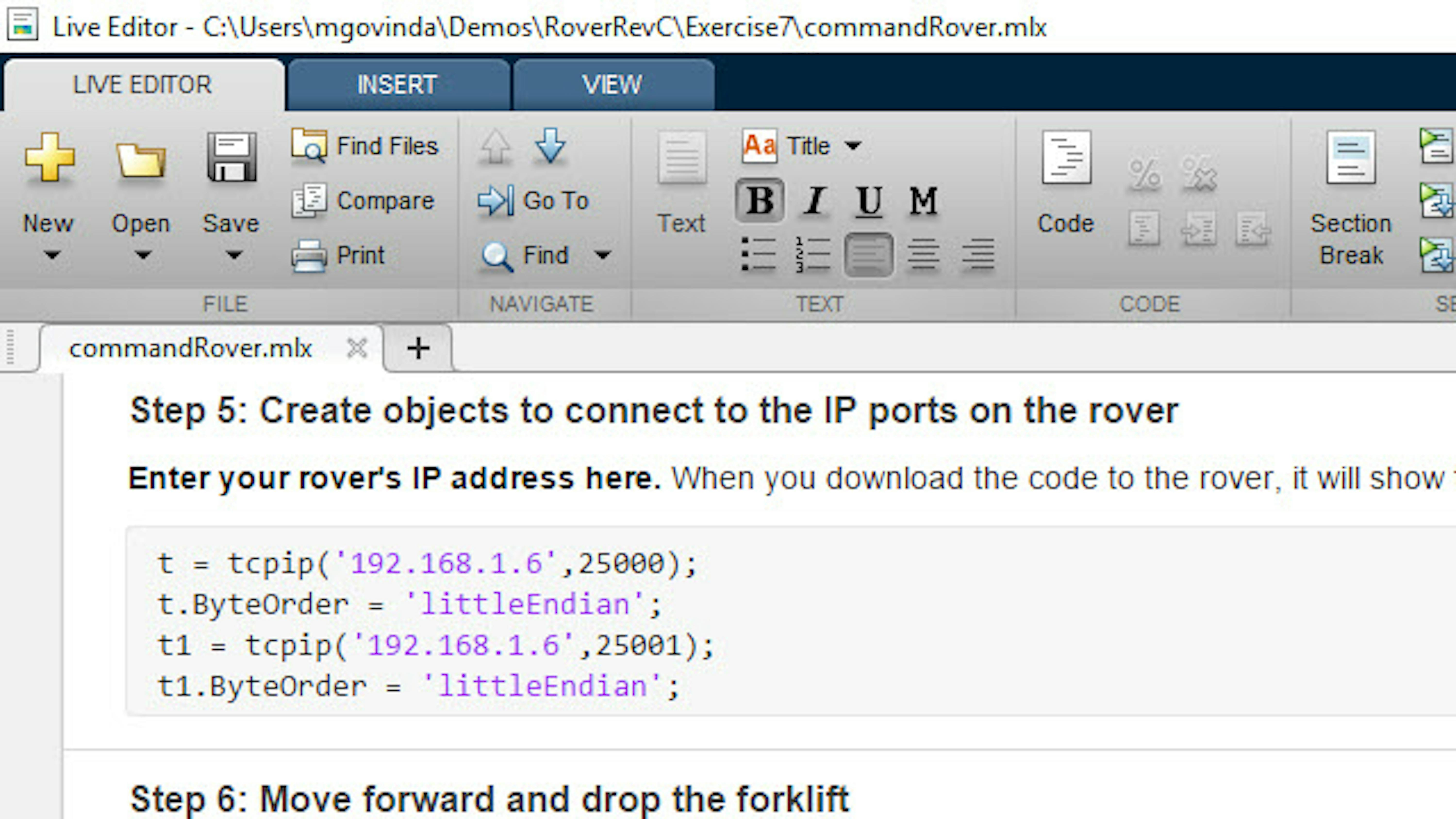
Note: Once these objects are created, you can send data to the specified IP ports using fwrite.
The section labeled "Step 6: Move forward and drop the forklift" is where the data is being sent from MATLAB to the deployed Simulink application over Wi-Fi. This step starts by defining a variable moveFlag that is used as input to the moveForward block. When moveFlag equals 1, the rover moves forward in the y-direction at 10 cm/s, and when it equals 0 the rover doesn't move.
moveFlag is initially set to 1 and conditional logic is used to instruct the rover to continue moving forward until the rover's y-location (as calculated by the localization algorithm, which runs once per second) is within 1 cm of the desired y-location.
Once the criterion is met, two things happen:
- moveFlag is set to 0 so that the rover stops moving forward.
- A for loop is used to move the forklift from the UP position (125 degrees) to the DOWN position (0 degrees).
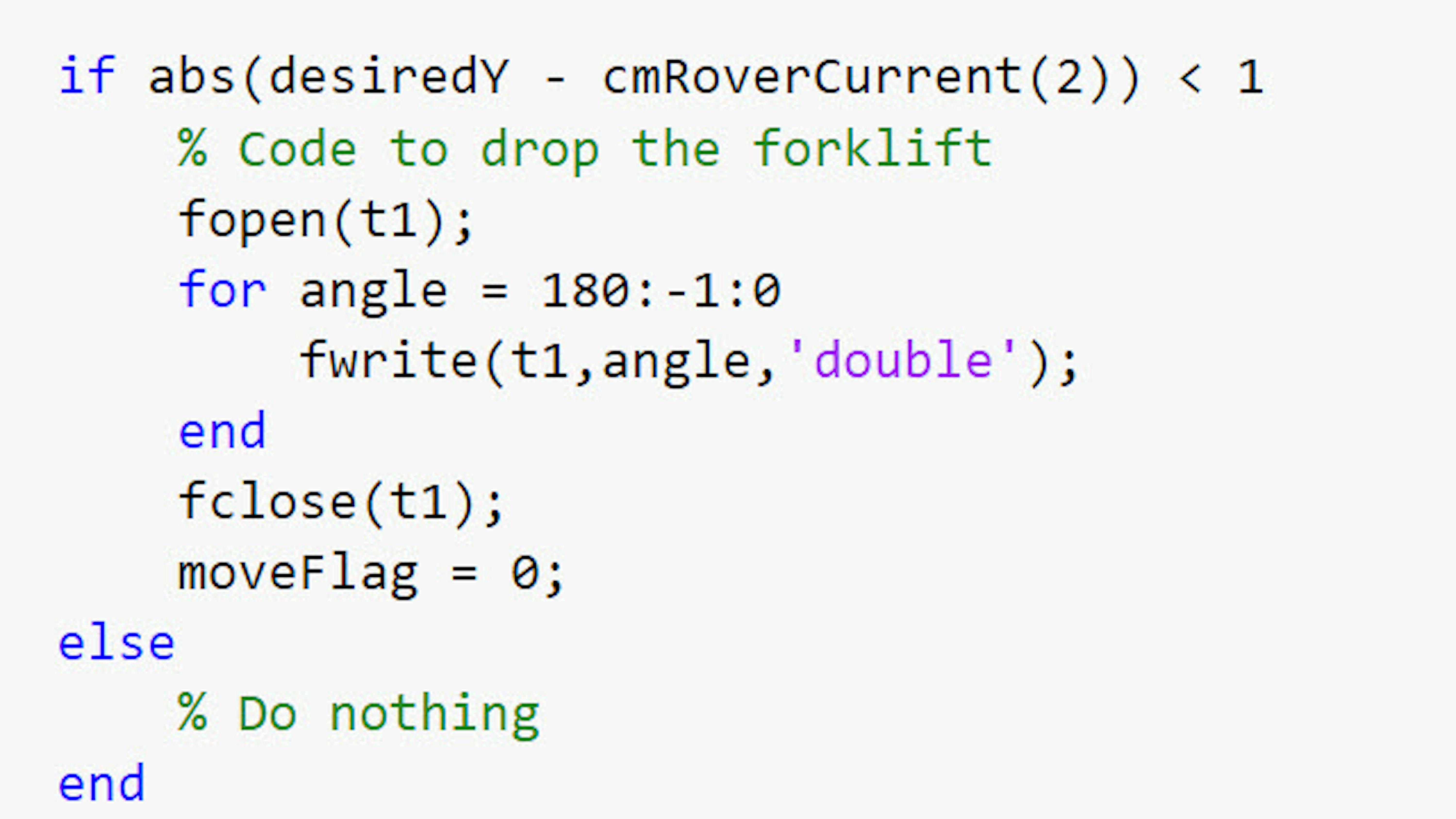
In summary, the MATLAB code uses Wi-Fi communication to instruct the rover to move forward to the desired y-location and then drop the forklift.
CONTROLLING THE ROVER FROM MATLAB OVER WI-FI
Now that you've learned about the Simulink models and MATLAB code, let's start controlling the rover from MATLAB.
Start by deciding on a place to put the rover on the arena. This must be a location where it's free to move forward at least 30 cm in the y-direction.
Important: As usual, if any aspects of your setup have changed (e.g., webcam or arena location, lighting), you need to recalibrate.
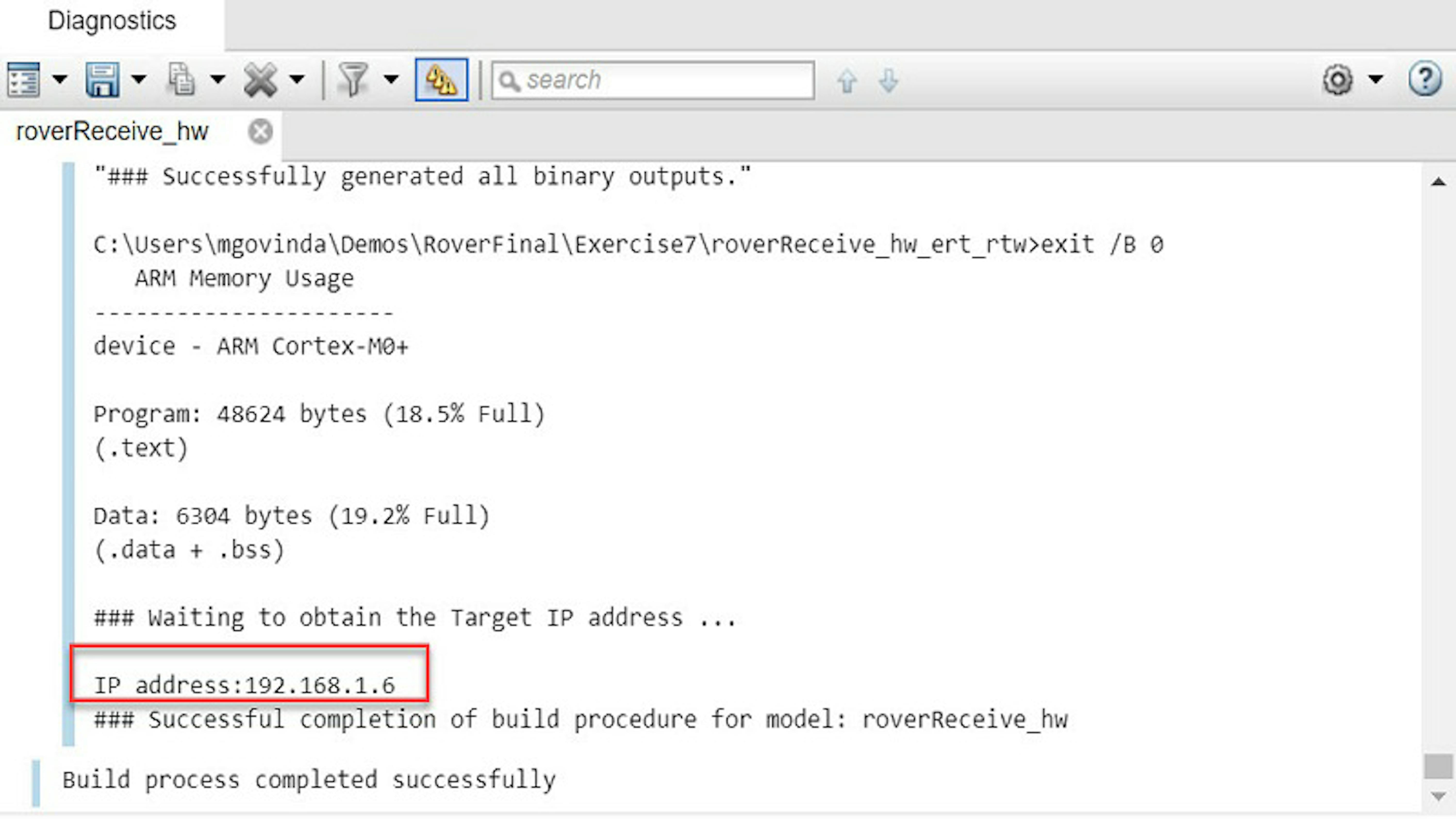
Deploy roverReceive_hw.slx to the rover. When the code generation is complete, click View Diagnostics to get your rover's IP address.
In the Diagnostics Viewer that opens, note the IP address of the rover.
Open commandRover.mlx and run the first four steps. Remember to follow any instructions within the Live Script.
Enter your rover's IP address in "Step 5: Create objects to connect to the IP ports on the rover" and click Run and Advance.
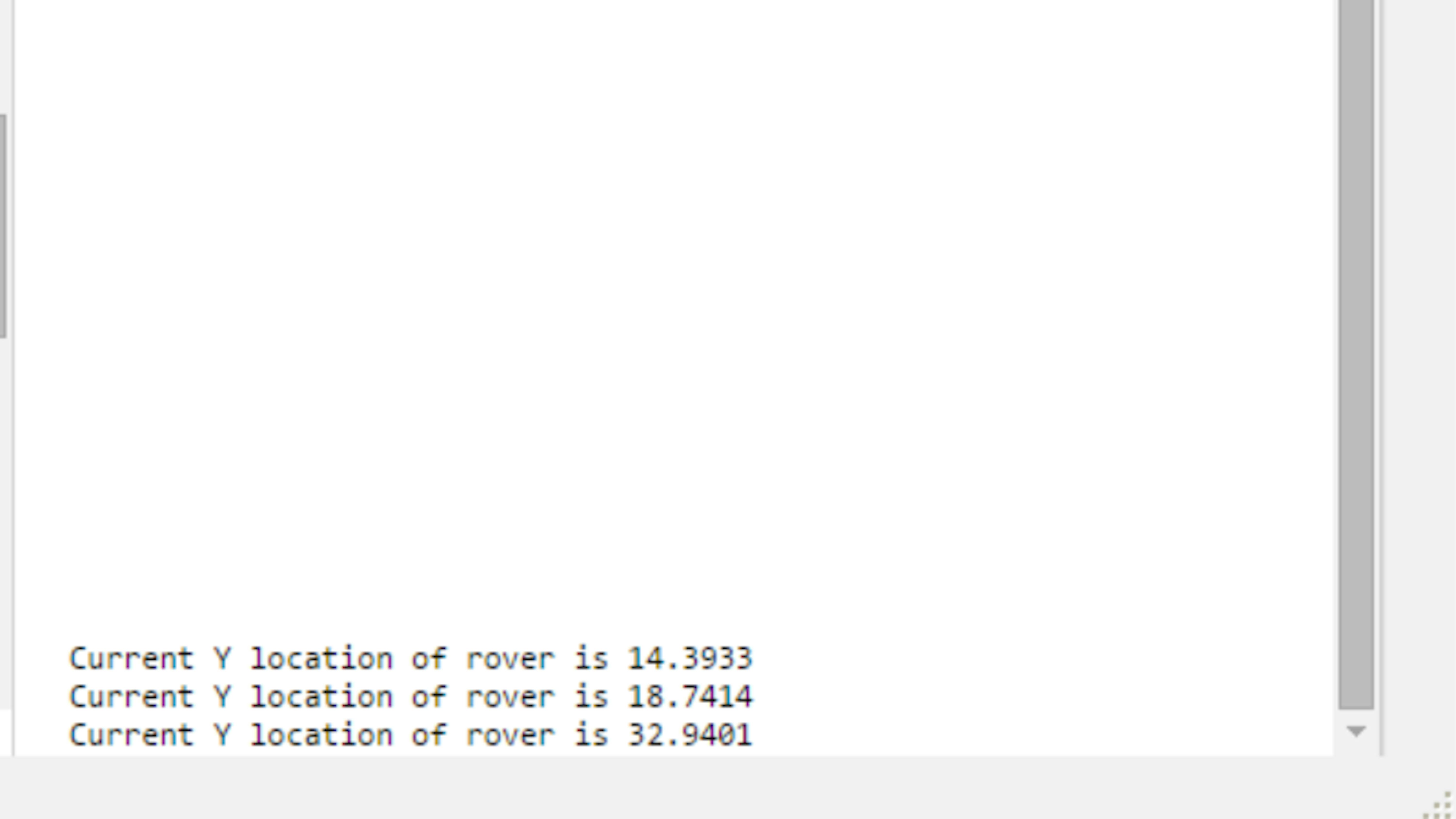
You will notice that the rover moves for approximately 1 second and stops. MATLAB calls the localization algorithm to calculate the rover's current y-location and displays it in the Output Window.
Once the rover has moved 30 cm in the y-direction from wherever it started, the forklift will drop. At this point, the application is complete.
SUMMARYREVIEW/SUMMARY
We saw how to communicate from MATLAB to the Rover and how to receive instructions over Wi-Fi on the rover.
FILES
-
roverReceive_hw.slx
-
commandRover.mlx
LEARN BY DOING
Add another Wi-Fi block to your Simulink model and update your MATLAB code accordingly so that you can command the rover to turn when needed.
5.8 Lessons learned
In this chapter you were introduced to a series of topics:
DIFFERENTIAL DRIVE MATH
The control of a differential drive robot. You had to physically build a simple two-wheeled rover carrying a mechanism (forklift) to lift and drop objects.
OPEN-LOOP VS. CLOSED-LOOP AND PID CONTROLLER
To get the rover to move, you learned about two possible strategies called open-loop and closed-loop. After discarding the open-loop controller that was just using information from the model of the motors under non-optimal conditions, you learned about how to implement a closed-loop controller using a PID controller using Simulink. While this strategy was a lot better than the open-loop controller, it still presented two undesired side effects: steady-state error and overshoot.
STATE MACHINES TO COMPENSATE ERROR
Once again, there is a way to avoid those two effects, in this case by using a state machine implemented with Stateflow, yet another toolbox within the MATLAB suite. Stateflow was also useful to create a simple program to control the forklift on the rover, which enables creating more challenging examples that include both moving the rover around, looking for an object at a desired location, and carrying it to yet another location. However, the initial conditions of the system were still an unknown: where was the rover located at the time of starting our MATLAB Live Script?
IMAGE PROCESSING TO HELP LOCATE OBJECTS IN REAL TIME
This final question is solved using a camera and an image processing algorithm that will look for the rover's RGB marker, which will help us to find the rover with pretty high accuracy on an arena of a predetermined size. We saw that this requires a complex calibration procedure that needs to be performed whenever the conditions change.
WIRELESS COMMUNICATION
Finally, using wireless communication, it is possible to have the rover in the same Wi-Fi network as the computer running MATLAB, which allows the rover to directly talk to Simulink and in that way open the possibility to a dynamic configuration mechanism.
5.9 Final challenge
Given all the learned lessons in this chapter, we are now ready to formulate a challenge including all the components of this module.
CONTROL THE ROVER USING THE LOCALIZATION ALGORITHM
Throughout the previous exercises, you saw how the rover can plan its path from a starting location to the target and finally to a specified endpoint location. One caveat with this approach is that there is no feedback on rover position other than the encoder data. If the wheels start slipping or the encoder data is noisy, you'll have problems.
It would be a good practice to have multiple sensors providing feedback on rover position to mitigate these potential issues. As you saw in Exercise 7, you can send signals from desktop MATLAB to a deployed Simulink model using Wi-Fi blocks. For the final challenge, implement a path-planning algorithm on the rover that uses the localization algorithm from Exercise 5 to provide additional feedback.
This is your final challenge. Go create an awesome mobile rover!