
Getting Started
Getting Started with Arduino, MATLAB, and Simulink
In this chapter, you will learn how to use the basic features from Arduino, MATLAB®, and Simulink® to make the projects in this kit work. Moreover, these tools are widely used, so you can apply everything you will learn in this chapter to all your future projects!
2.1
Arduino getting started
In this section, you will learn:
- How to install and configure the Arduino IDE.
- About the Arduino MKR1000 board.
- How to use digital inputs/outputs and serial communication with Arduino.
- How to use Arduino Carriers together with Arduino boards.
- About the Arduino MKR Motor Carrier.
- To move a motor by using the Arduino MKR Motor Carrier.
ARDUINO BOARDS FAMILY
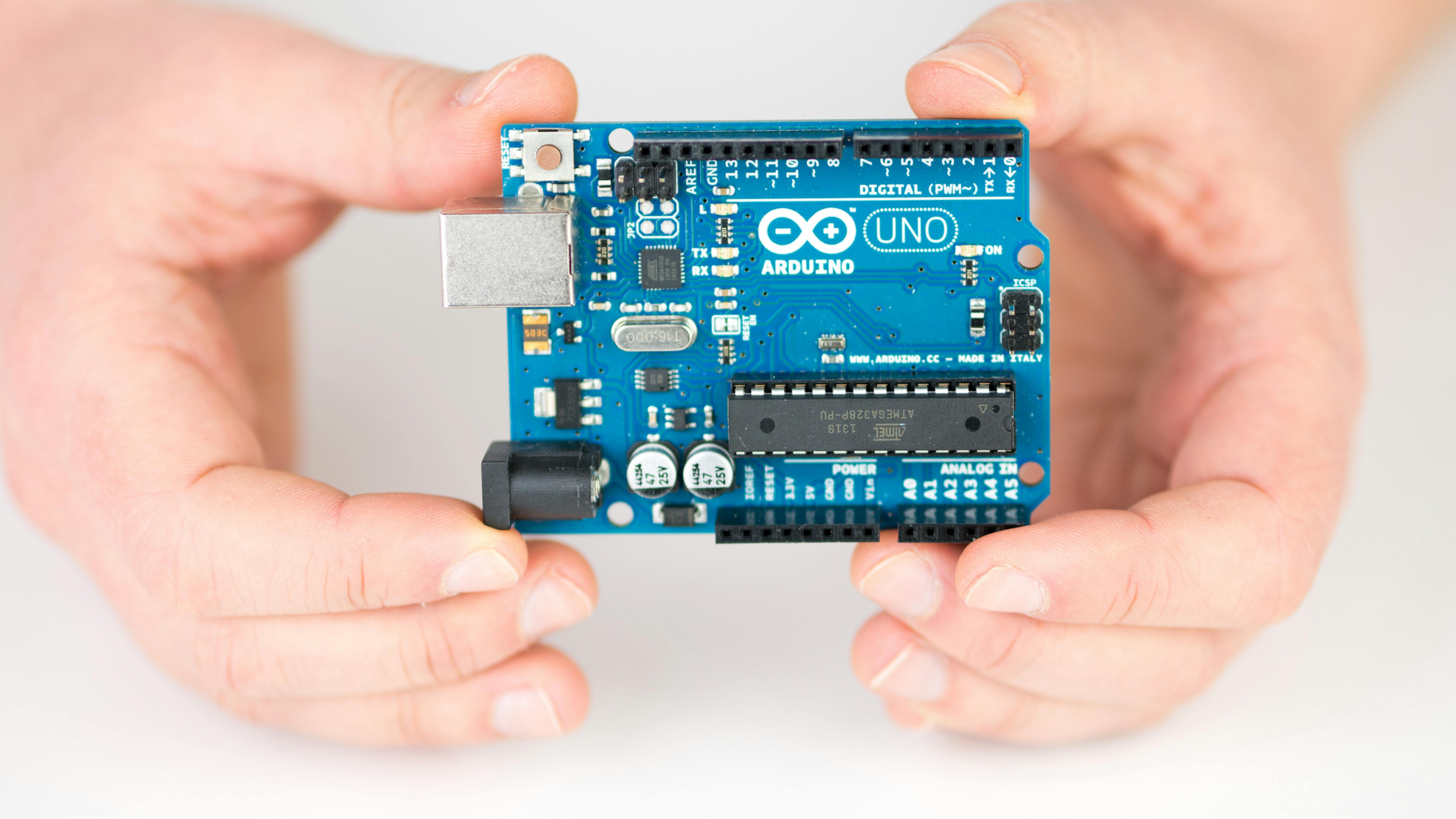
Over the years, Arduino has developed a variety of boards , each one with different capabilities and functionalities. For instance, there is a different MKR board for each communication protocol, such as Wi-Fi, Bluetooth, LoRa, SigFox, GSM and so on. The most popular board for beginners is the Arduino UNO. Based on the ATmega328P processor from ATMEL, it is the most used board of the whole Arduino family, as well as the most robust, perfect for getting started at tinkering with the platform.
Boards released after the UNO up to 2017 have more advanced processors with more memory and enhanced input/output features, but for the most part they use the same pinout arrangements and will work with existing add-on boards, called Shields or Carriers, and various add-on components such as sensors, communication chipsets, and actuators.
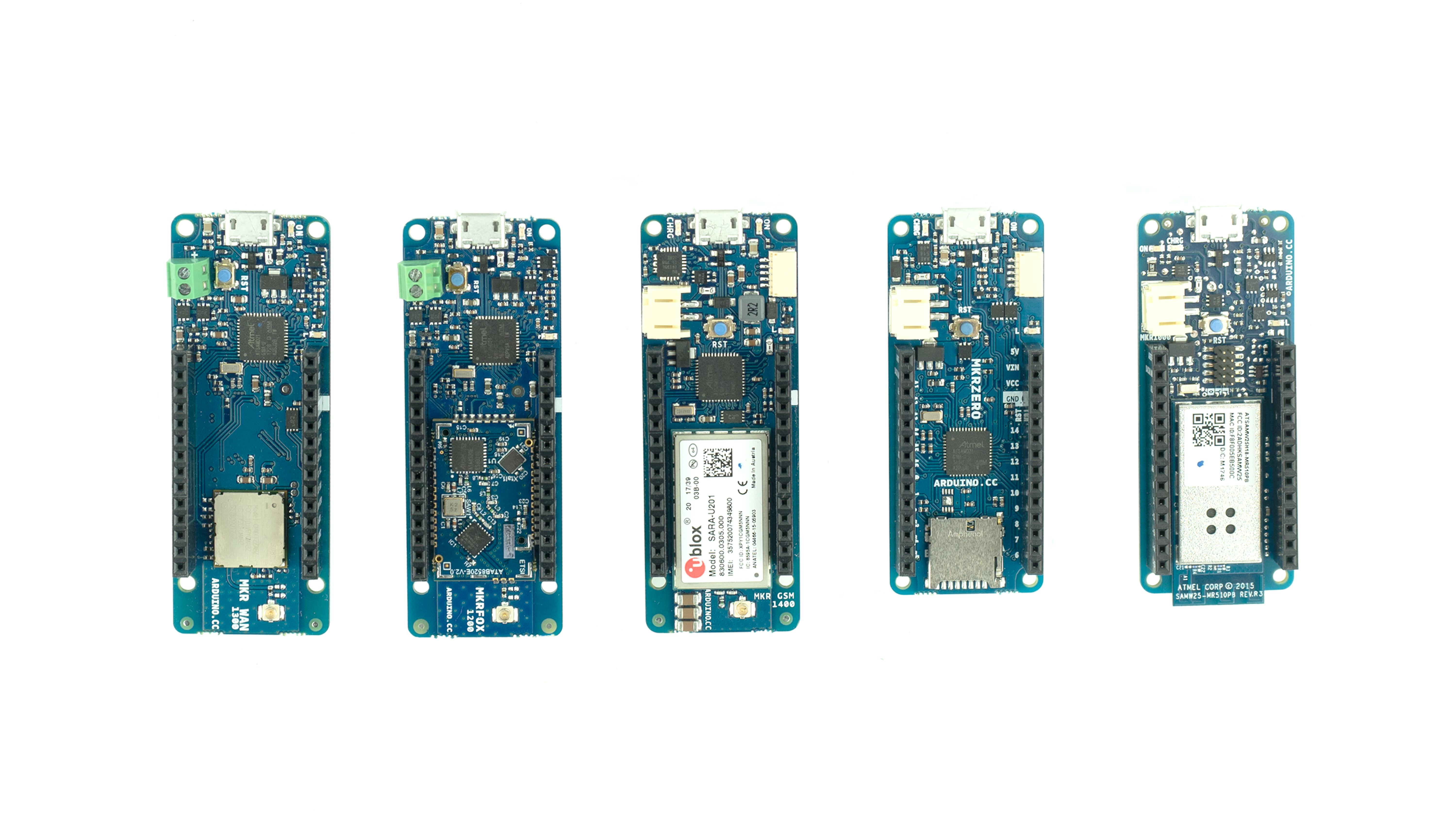
In 2017, Arduino released the MKR1000 board, an entirely new design establishing a new standard in terms of pinout, shape, and operating voltage (3.3 V). After that, several boards have been released following this new standard to create a new subset of Arduino boards called the MKR family. As explained earlier, this family of boards is made for those who need a specific digital communication protocol (Wi-Fi, Lora, SigFox, etc.) while keeping the classic Arduino boards' ease of use.
ARDUINO MKR1000 BOARD
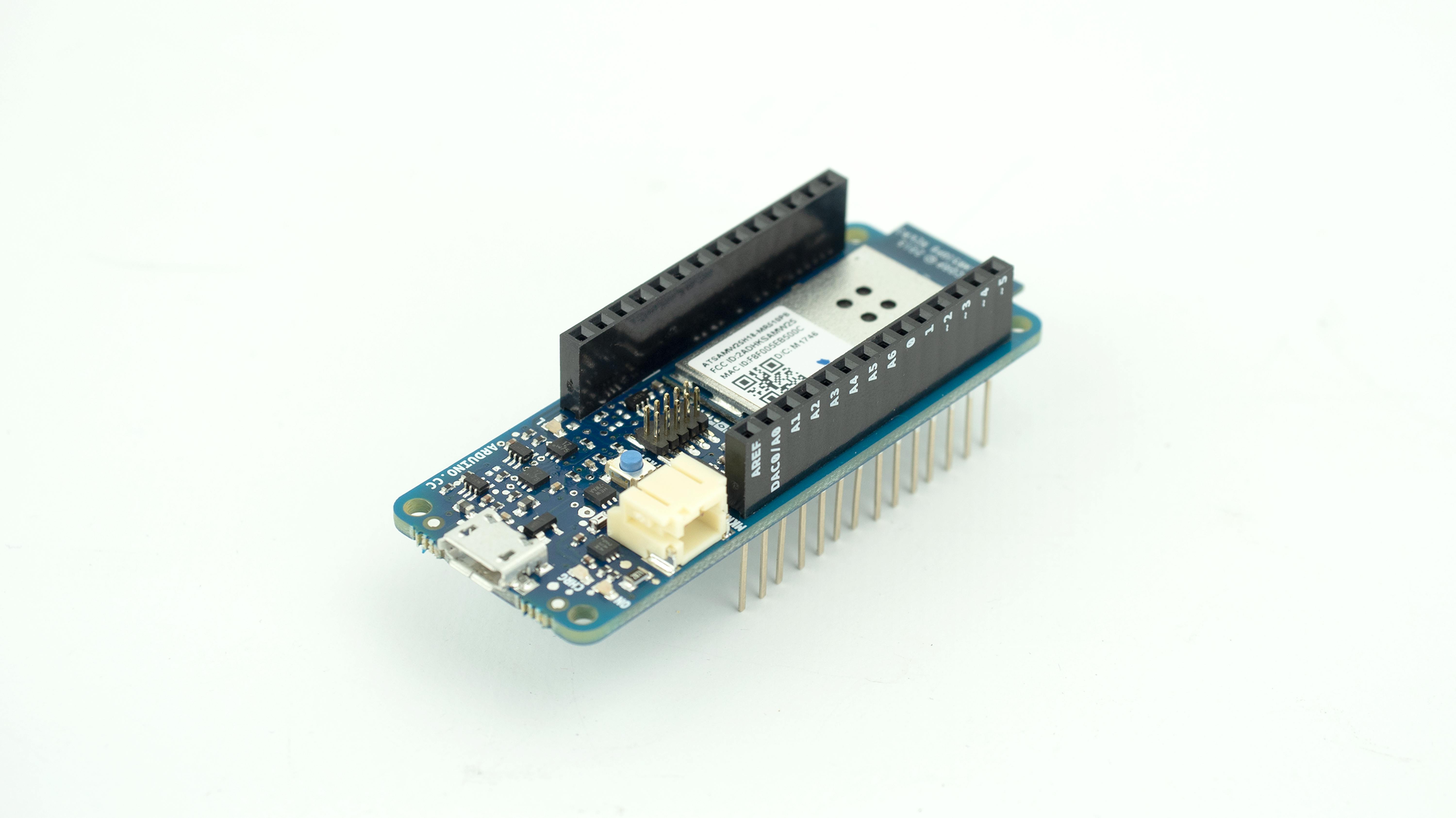
The Arduino MKR1000 is a powerful board based on the Atmel ATSAMW25 SoC, which has been designed to offer a practical and cost-effective solution for makers seeking to add WiFi wireless connectivity to their projects.
First of its family, the MKR1000 is a versatile board: it includes a LiPo charging circuit that allows it to run on batteries, has a WiFi module with a crypto-chip to ensure secure communications, and can be configured to constrain its power consumption to keep it running for long periods.
The WiFi connectivity makes it the perfect board for any project related to the Internet of Things. It allows communication with hundreds of online services that offer RESTful APIs, such as Twitter, GitHub, IFTTT, or Telegram, to name a few. The board can also be used as a WiFi access point, creating a local network that can run a small web server hosting websites and online interfaces.
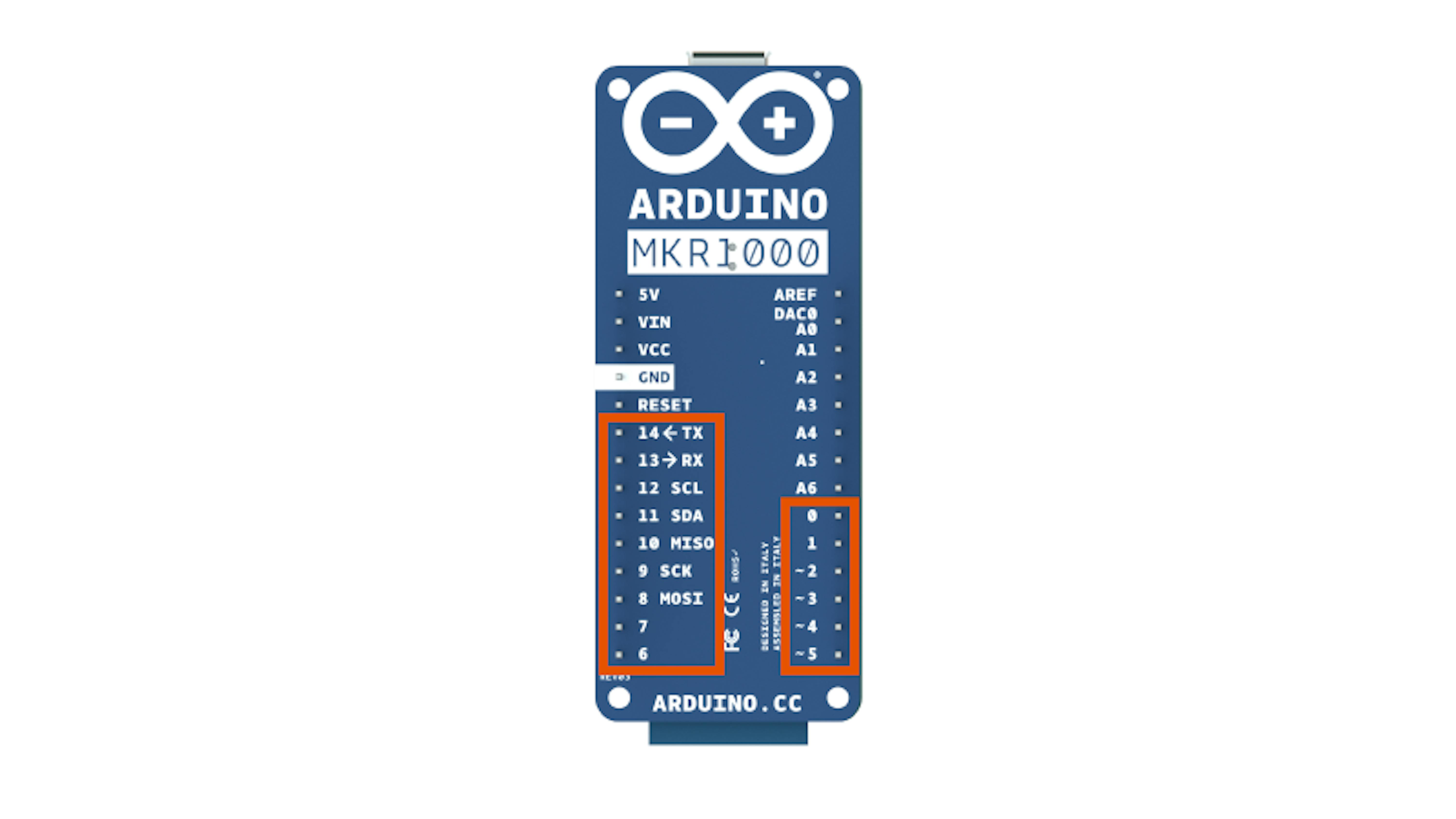
The MKR1000 board has 28 pins, some of which have fixed functionalities and some of which have configurable functionalities. Fixed functionality pins include GND and 5V, which provide access to the board's ground and 5-volt reference voltage lines respectively. The pins labeled A0 to A6, are analog pins. These pins can transmit or receive voltage values between 0 and 3.3 volts, relative to GND. Finally, the pins labeled 0 to 14 are digital pins. When these pins transmit data, they can only transmit voltage values of 0 or 3.3 volts, relative to GND. When they receive data, the voltage is interpreted as HIGH or LOW, relative to some threshold between 0 and 3.3 volts. Note that you must never apply more than 3.3 volts to the board's digital and analog pins. Care must be taken when connecting sensors and actuators to assure that this limit of 3.3 volts is never exceeded. Connecting higher voltage signals, like the 5V commonly used with the other Arduino boards, will damage the MKR1000.
WORKING WITH DIGITAL OUTPUTS
The pins on the Arduino boards can be used to control and communicate with external components, such as LEDs, motors, or sensors. Pins can be configured either as INPUT or OUTPUT. Pins configured as INPUT enable the board to read values from external components attached to the pin, such as the light intensity from a phototransistor or the state of a button. When pins are configured as OUTPUT, the board will be able to control and communicate with actuators, lighting up an LED or playing sound on a buzzer.
Pins configured as OUTPUT are said to be in a low-impedance state. In this configuration, the pin can provide current to other circuits. Output pins in the MKR1000 can source up to 7 mA (milliamps) of current per I/O pin to other devices and circuits. This means that you cannot, for example, drive a motor directly from a pin because the current will not suffice. You will need to consider the use of drivers of different types to achieve different tasks like lighting up high power LEDs, driving motors, or activating relays.
Digital pins can only have two states, ON and OFF or, as labeled in the Arduino programming language, HIGH and LOW. We use the digitalWrite() function to set a pin to the desired state , indicating between the brackets which pin we want to act upon and the state we want it to be in.
INSTALL THE ARDUINO IDE
To test the MKR1000 board included in the kit, you need to install the Arduino IDE. There are two different versions of the IDE: the classic offline Java IDE, and the newer cloud-based Create IDE. At the time of writing, the interaction between MATLAB and Arduino is possible only through the classic IDE and therefore the following explanations will be about configuring this specific tool. The classic Arduino IDE can be downloaded from the following link. Choose the version corresponding to the operating system in your computer and follow the instructions. This page in the Arduino server will give you more information about this process.
The classic Arduino IDE is a relatively small download (about 100 MB) and is tailored to suit the needs of traditional Arduino users, who typically own an Arduino UNO, Nano, or Micro board. However, the Arduino MKR family needs a different toolchain, the set of tools to produce binary executables for Arduino from code, that is a lot heavier and that must be downloaded separately. This operation is very simple and can be done directly from within the IDE. The whole operation is described in Arduino's getting started guide to MKR1000, which you can find here.
By installing the necessary files to compile programs for the MKR1000, you will also install the drivers needed for your computer to identify the board and communicate with it. The three main operating systems, Windows, Linux, and Mac OSX, handle the connection of new USB devices differently. In Windows, Arduino boards are typically listed as serial ports and labeled with the term COM followed by a number. In Linux, the boards show up as a peripheral under the /dev/ folder, more specifically /dev/ttyACM and a number. Finally, Mac OSX detects Arduino boards under the /dev/tty.usbmodem descriptor (also followed by a number). For more in-depth explanations of how to troubleshoot possible issues arising when trying to detect the boards, please check the getting started guide for the MKR1000 once more, or contact the Arduino support line if you need more help.
CONNECT THE MKR1000 TO YOUR COMPUTER USING THE USB CABLE AND TRY IT OUT

Let's make sure the installation of the IDE and drivers was successful by trying out the simplest example included with the Arduino IDE. The so-called Blink example (open it at File>Examples>Basics>Blink), will be turning the on-board LED on and off in an endless loop.

All Arduino boards have an on-board LED connected to one of the digital pins, although the location may vary from board to board. On the MKR1000 the LED is connected to pin number 6, while on the classic Arduino UNO board it is connected to pin 13. The Arduino programming environment has a system constant called LED_BUILTIN that represents the LED pin for the specific board being programmed. Let's take a quick look at the code for this example:
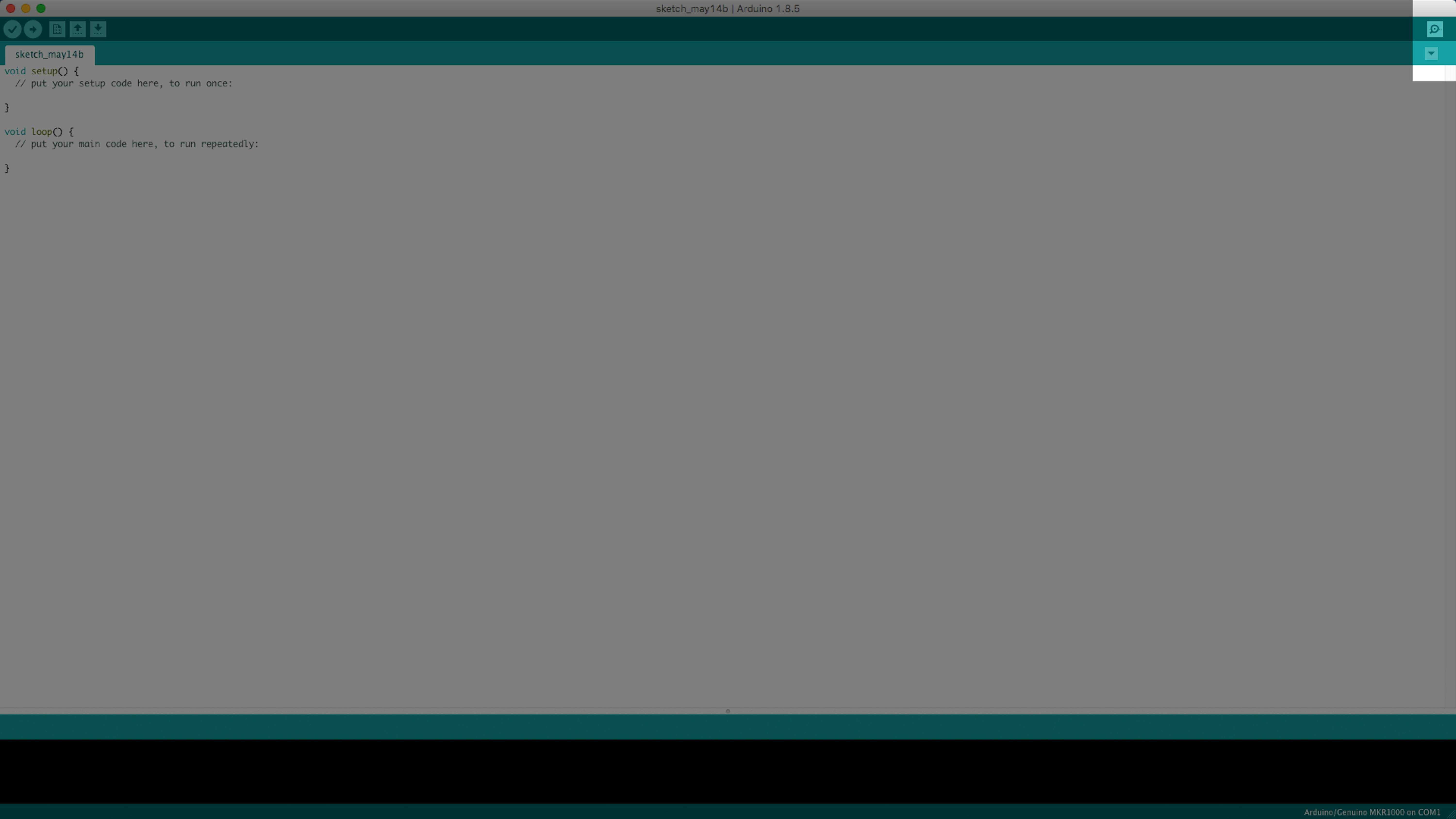
The setup() function contains instructions that must be executed only once as a way to configure the board. In it, we set the pin attached to the LED as an OUTPUT using the function 'pinMode().'
The loop() function contains instructions that will be looped consecutively. As you can see, we first turn on the LED by setting the pin to the HIGH state and then turn it off by setting the pin to LOW.
Between those two pin-writing actions the delay() function will stop the program from being executed for the amount of milliseconds indicated in the brackets. This enables us to see the LED changing state, since otherwise the change would be too fast to be perceived by the human eye. Upload the Blink example to the board to see the result. Instead of using the built-in LED, you could connect an external LED and use whatever digital pin you want.
Note: Remember to separate the conductive foam from all the boards before you start experimenting with them.
WORKING WITH DIGITAL INPUTS
Arduino pins are configured as INPUT by default. Pins configured this way are said to be in a high-impedance state. Input pins could be modeled as if they had a 100 Mohm resistor in series in front of the pin. This means that it takes very little current to get the input pin to change from one state to another. Pins, when configured as inputs, are useful for reading values of buttons, switches, and more generally all those sensors that have only two states: ON or OFF.
To read values from a pin configured as INPUT we use the digitalRead() function, indicating between the brackets which pin we want to read values from. The function returns a value that can be either HIGH or LOW (which corresponds to the integers 1 or 0). Open the Button example in the Arduino IDE (located in the menu File>Examples>Digital>Button) and look at it. The following image shows the example opened in the IDE.
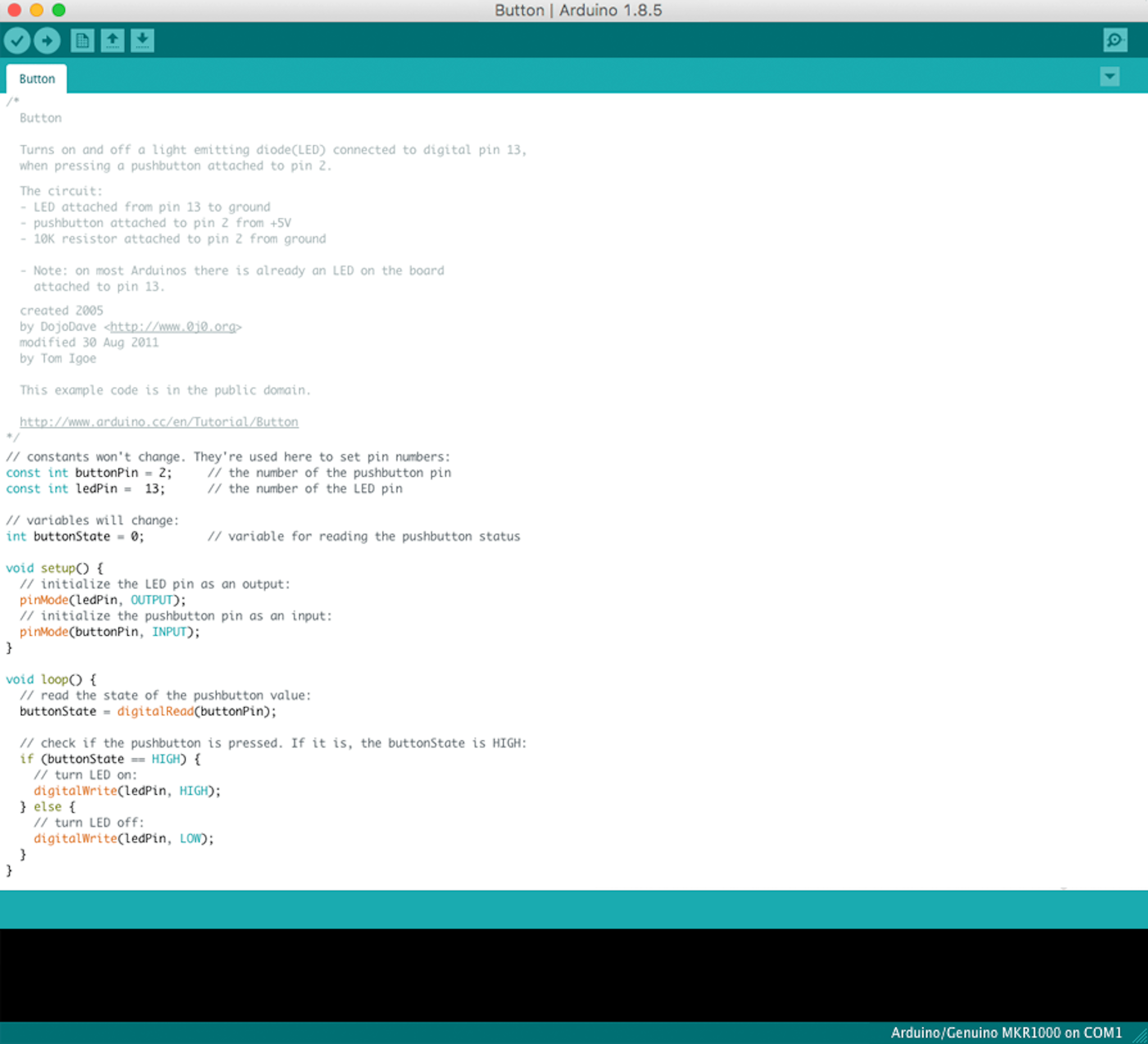
In this example, we first declare the variables we will use, such as buttonPin and ledPin; these are just human-readable names we can give to the pins connected to the button and to the LED. There is a third variable, called buttonState, that will be used to store the value returned from reading the pin connected to the button.
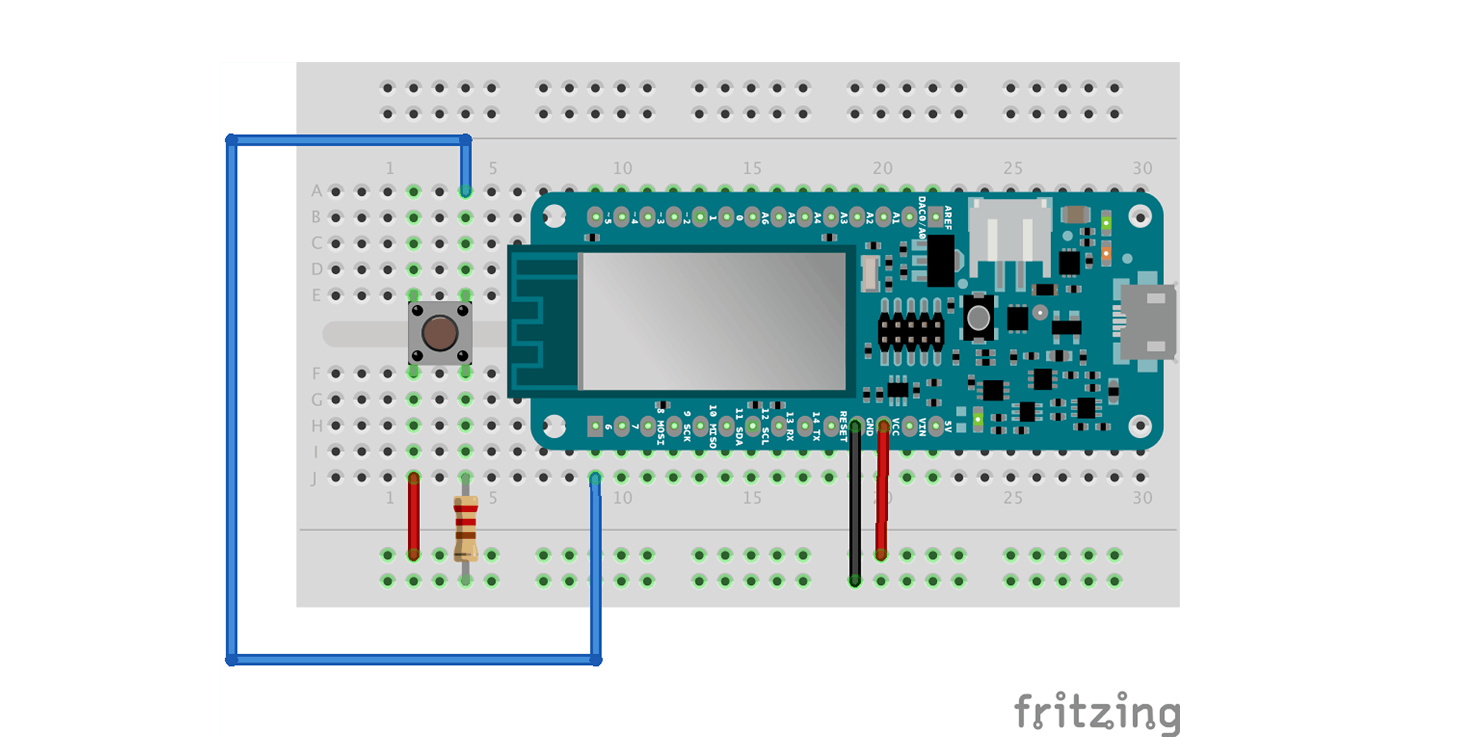
Note: To try the code, we will suggest that you build a circuit, and you will need to change the code to correspond to the circuit. In the illustration that follows, the button will be connected to pin number 6, so you will have to change the initial declaration of buttonPin to correspond to this case. We then read the state of the button and store it in buttonState as you can see in the following code snippet:
Using an if statement, we can then turn the LED ON or OFF according to the state of the button., ON if the button is pressed and OFF if it is not.
COMMUNICATING TO ARDUINO VIA SERIAL
Arduino boards communicate with computers and other devices via serial communication. All Arduino boards have at least one serial port (also known as a UART or USART). Serial data consists of a series of 1's and 0's sent over the USB cable at a certain speed. Data can be sent both from the board to the computer and vice-versa.
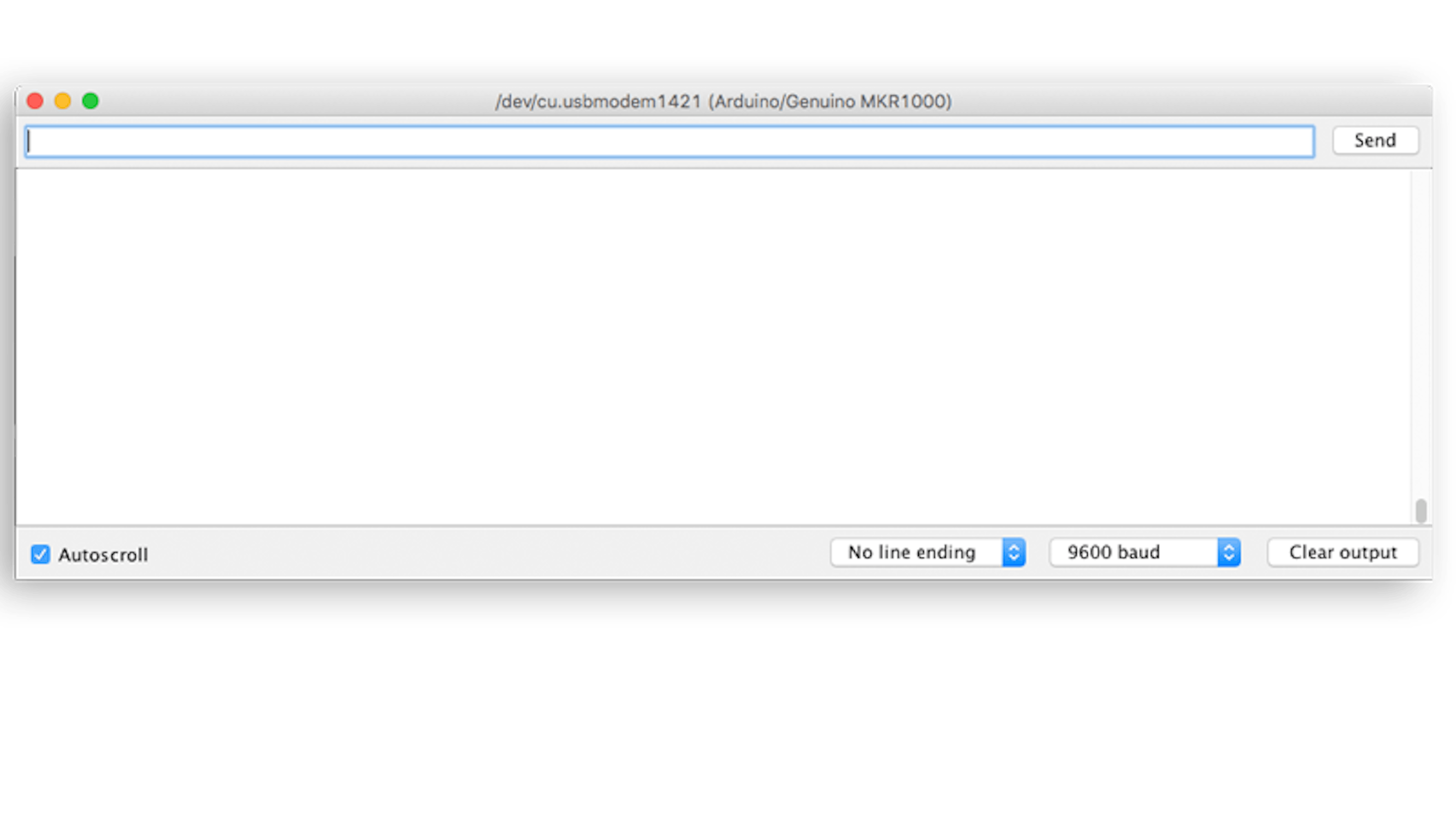
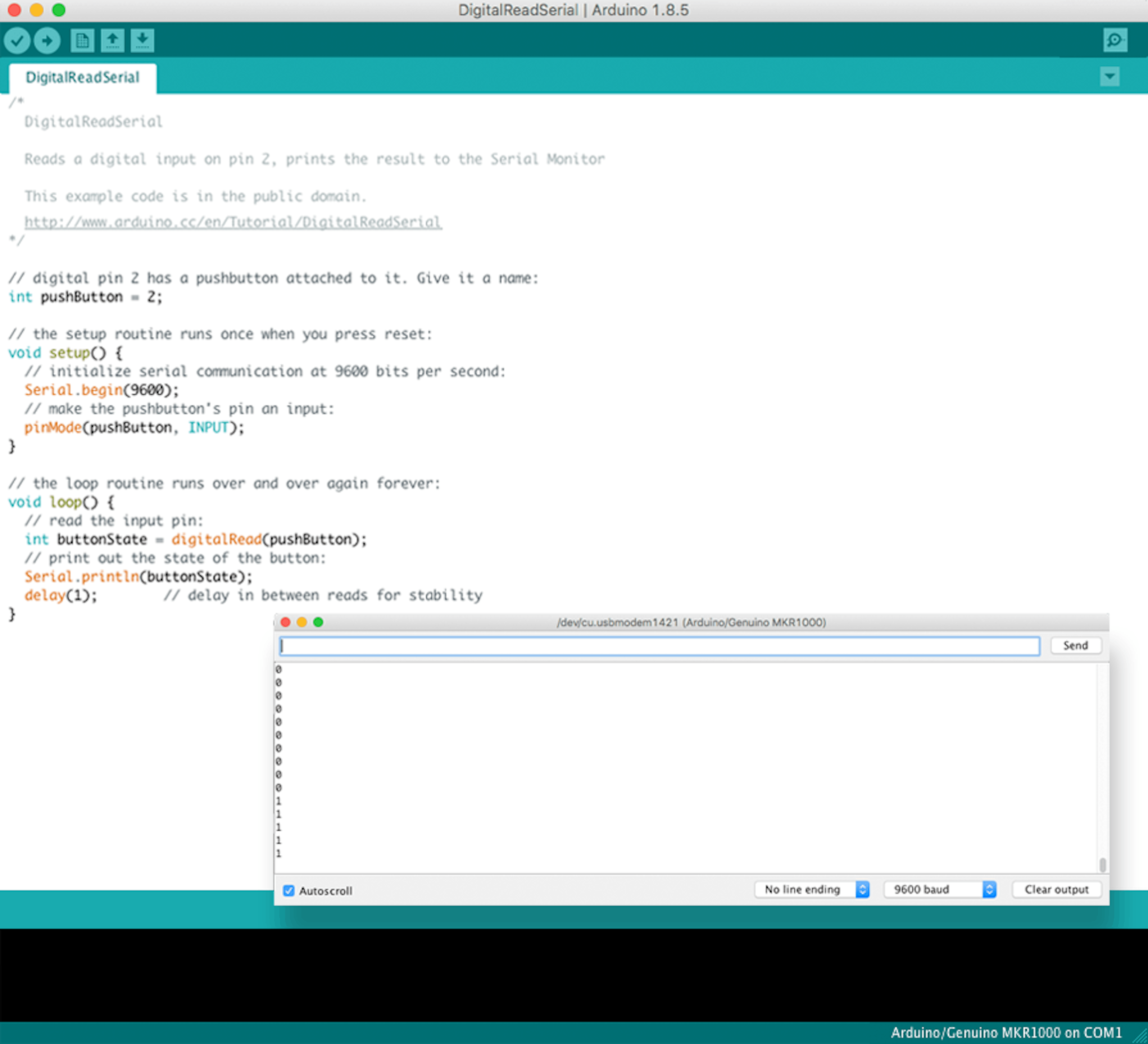
The Arduino IDE as well as the Create Editor hasve a feature called the Serial Monitor, that is of great help when debugging sketches. (Sketch is the way we call to Arduino programs.) The Serial Monitor is a pop-up window in the classic IDE acting as a separate terminal that communicates by receiving and sending serial data; you invoke it by pressing the magnifying glass icon at the right side of the toolbar on the IDE. The Create Editor has the Serial Monitor implemented as a layer that overlays part of the editor dedicated to displaying the file navigation. 
To use serial communication with Arduino, we first need to initialize it by calling the function Serial.begin(). Between the brackets we type the baud rate, which is the data rate in bits per second (baud) for serial data transmission. The most common baud rate used is 9600. You should be aware that different devices and systems communicate at different speeds, so you need to configure both ends of the communication (emitter and receiver) to operate at the same ratio of bits per second.
Try out how the serial port works through an example. Open the DigitalReadSerial example ( File>Examples>Basics>DigitalReadSerial ) and check the code.
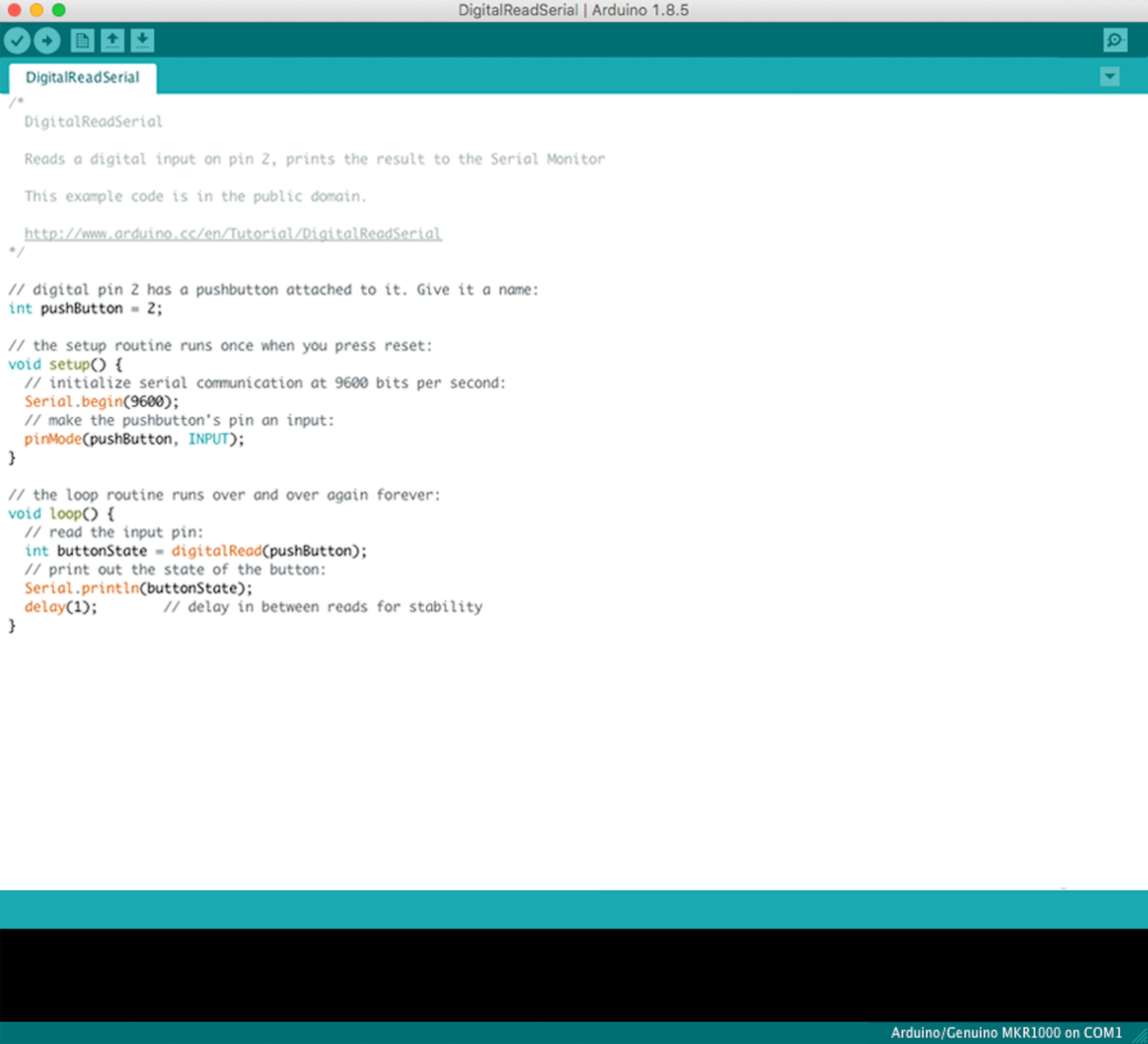
This example illustrates how to read values from a button connected to pin number 2 and print those values on the Serial Monitor using the Serial.println() function.
Depending on whether the button is pressed, a 0 or a 1 will be printed on the console. The circuit configuration is the same as the button example used earlier in the chapter.
ARDUINO SHIELDS/CARRIERS
Shields/Carriers are boards that can be plugged on top or underneath an Arduino board to extend its capabilities. They are generally used to simplify connecting sensors and actuators that either require a lot of electronics to be implemented, that exist only as surface mounted components, or that are used very often.
Since there are different Arduino boards with different pinouts and shapes, there are different Shields/Carriers as well. The main difference is between the old Arduino family (based on the UNO pinout) and the new MKR family. It is also possible to use the shields made for the older boards with the newer ones by using a simple adapter Shield. An example of a shield made for the MKR1000 family is the MKR relay proto shield that you can see in the following image:
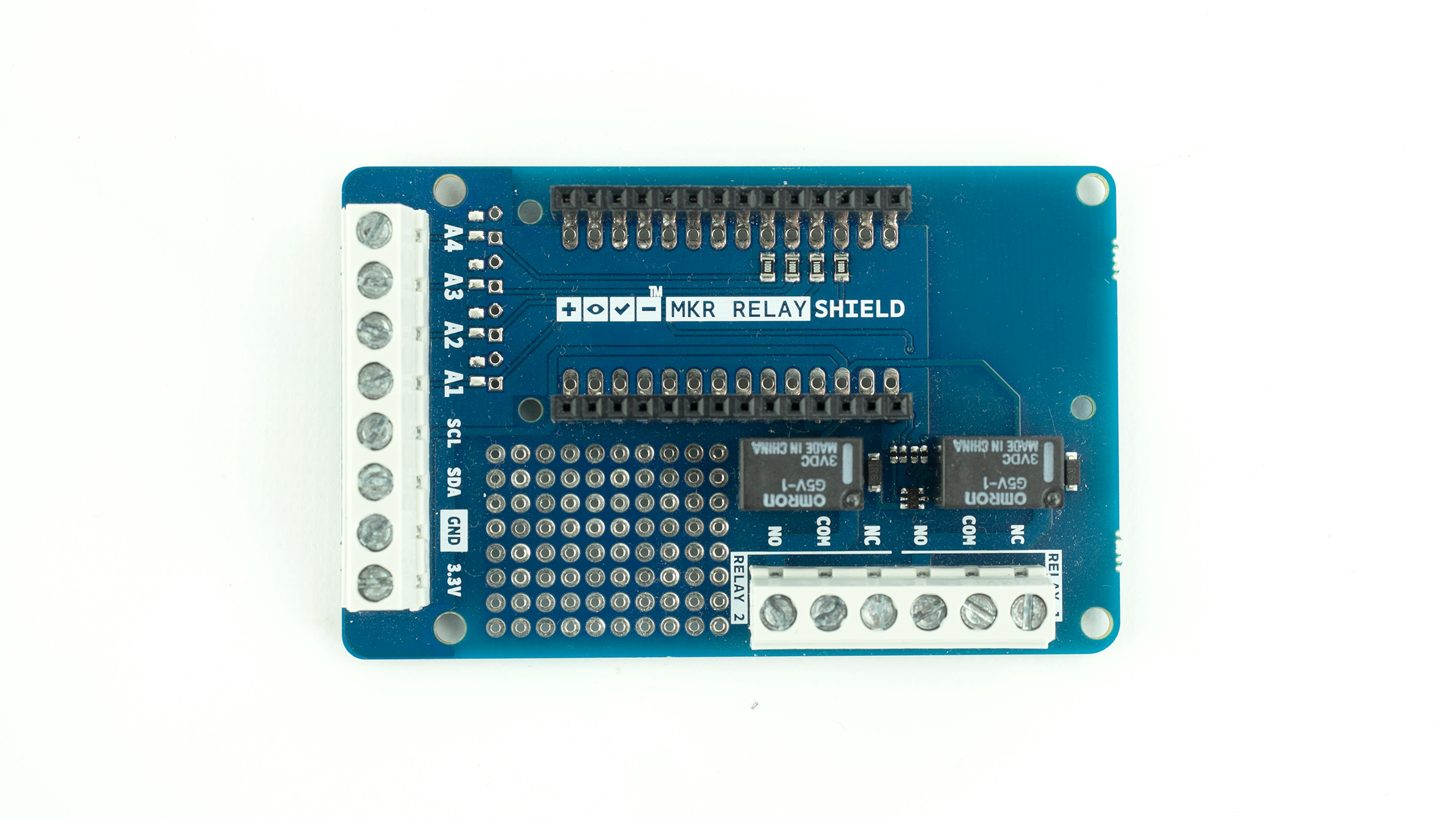
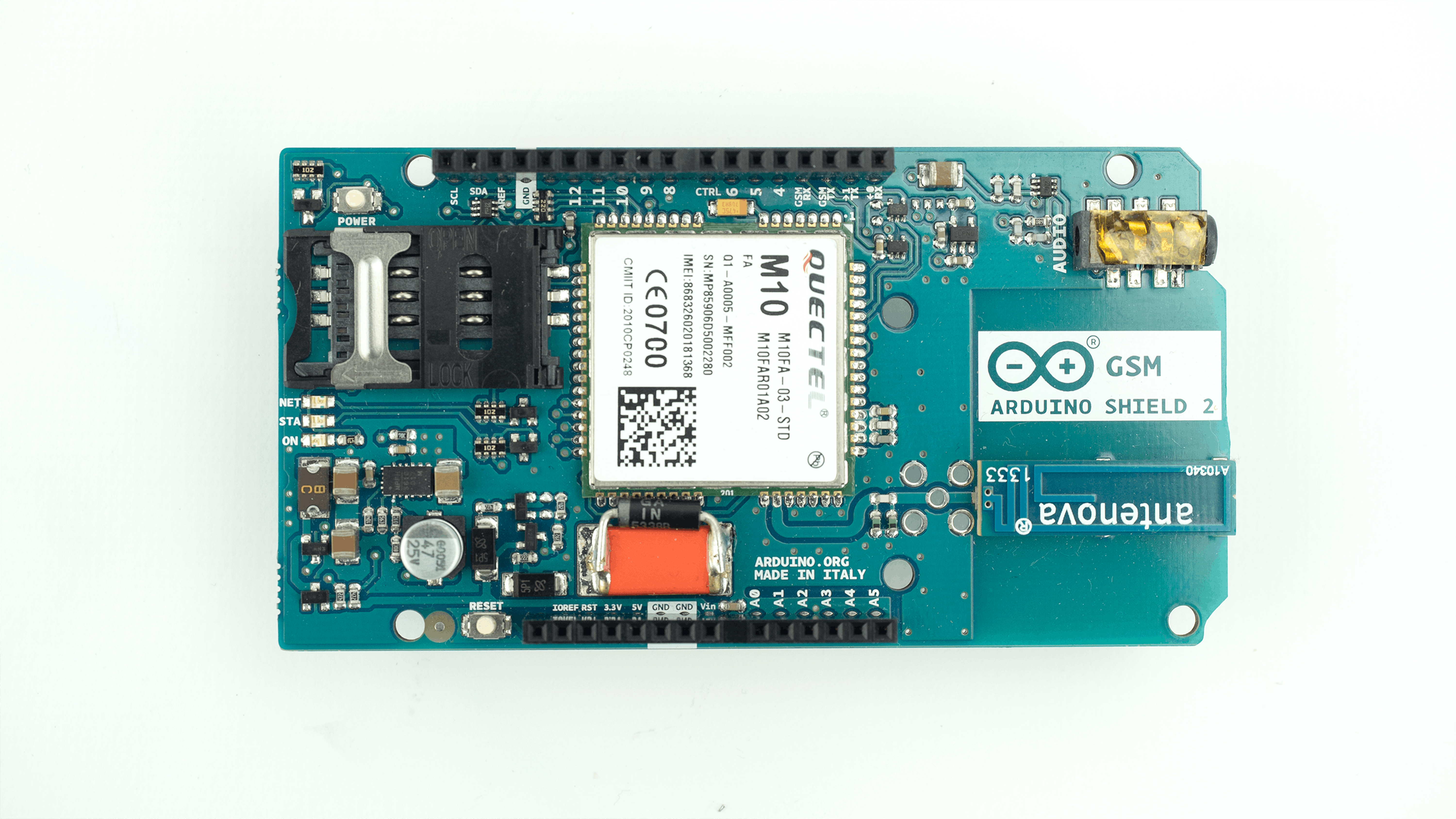
The MKR Relay Shield can be plugged underneath any board of the MKR family, allowing you to easily control two relays without the effort of wiring them up. Other shields add communication capabilities to the boards. The GSM Shield, for instance, allows the Arduino board to make phone calls, send SMS messages, and connect to the internet.
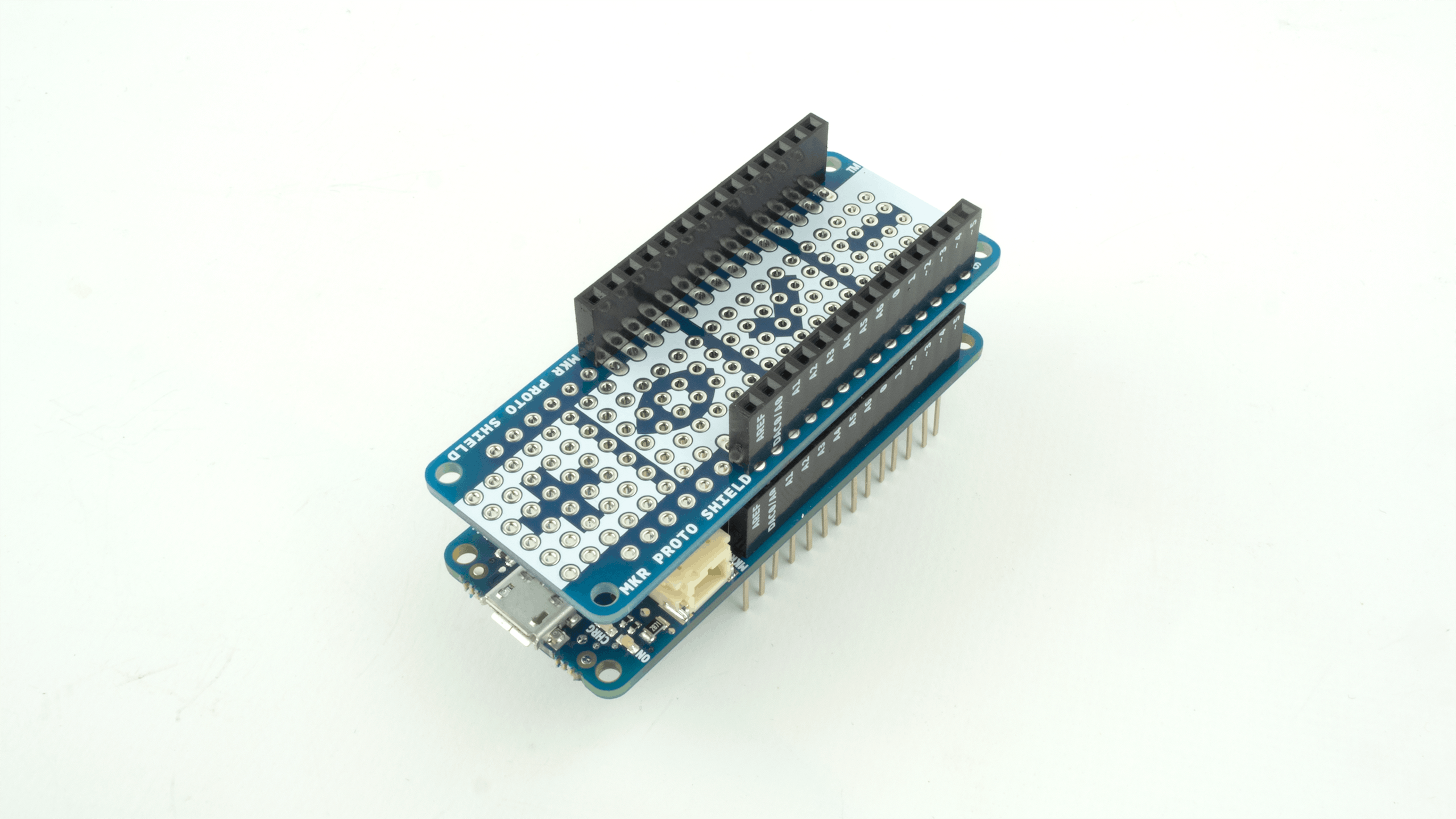
Another kind of shield that sometimes comes in handy is the MKR Proto Shield. This is a shield that offers space to solder components onto it, making the project more compact and robust.
While some of the above-presented Shields add the possibility of connecting sensors or actuators in an easier way, others include complex devices that require extra blocks of code to handle them. Thus, some Shields (such as the GSM one) come with new libraries of code that must be added to the IDE. You can read more about how to find and add new libraries to your Arduino IDE at this link.
This section has introduced you to the idea of Shields; the next section will present the Carrier that was created especially for this kit, the MKR Motor Carrier.
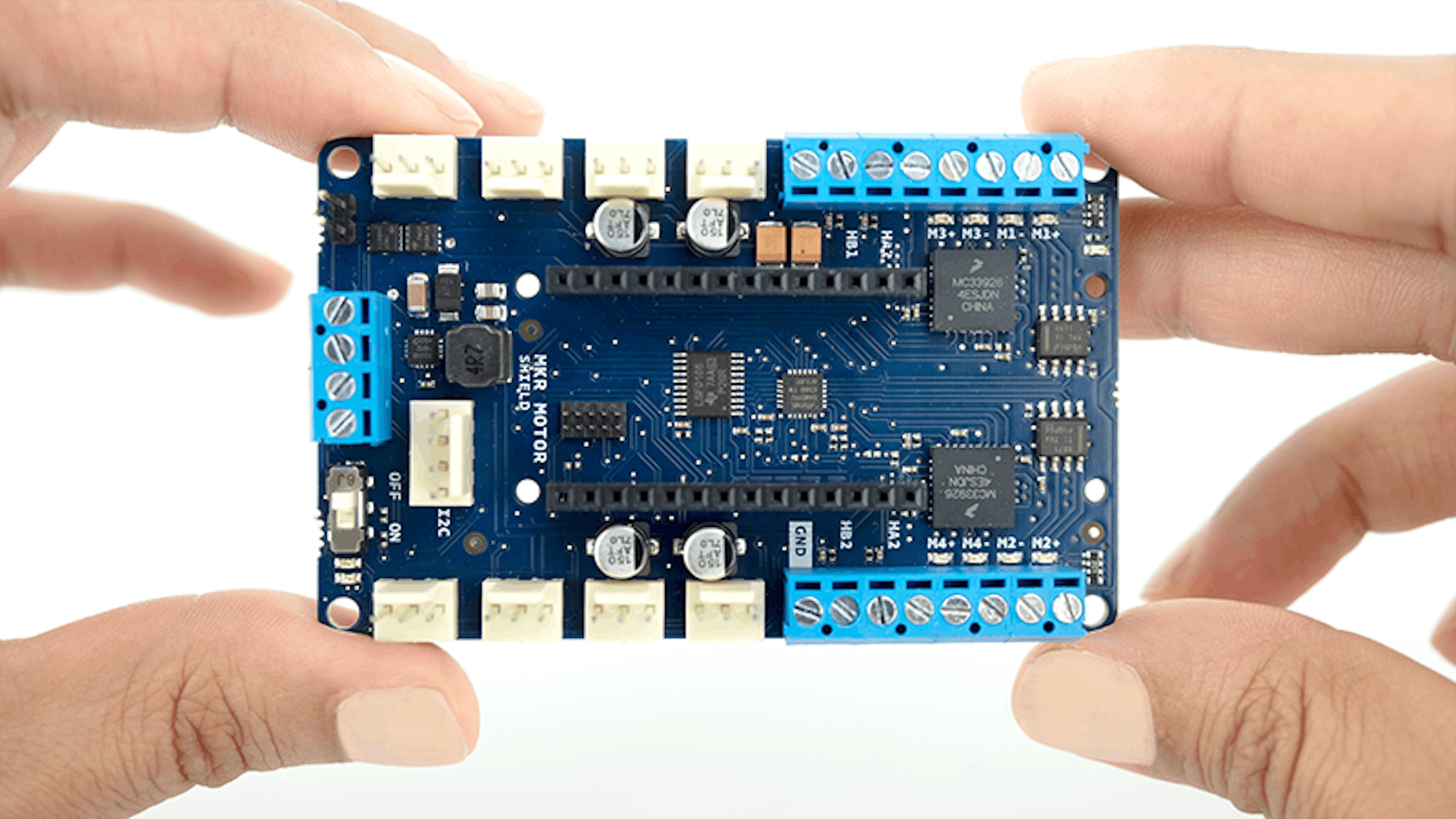
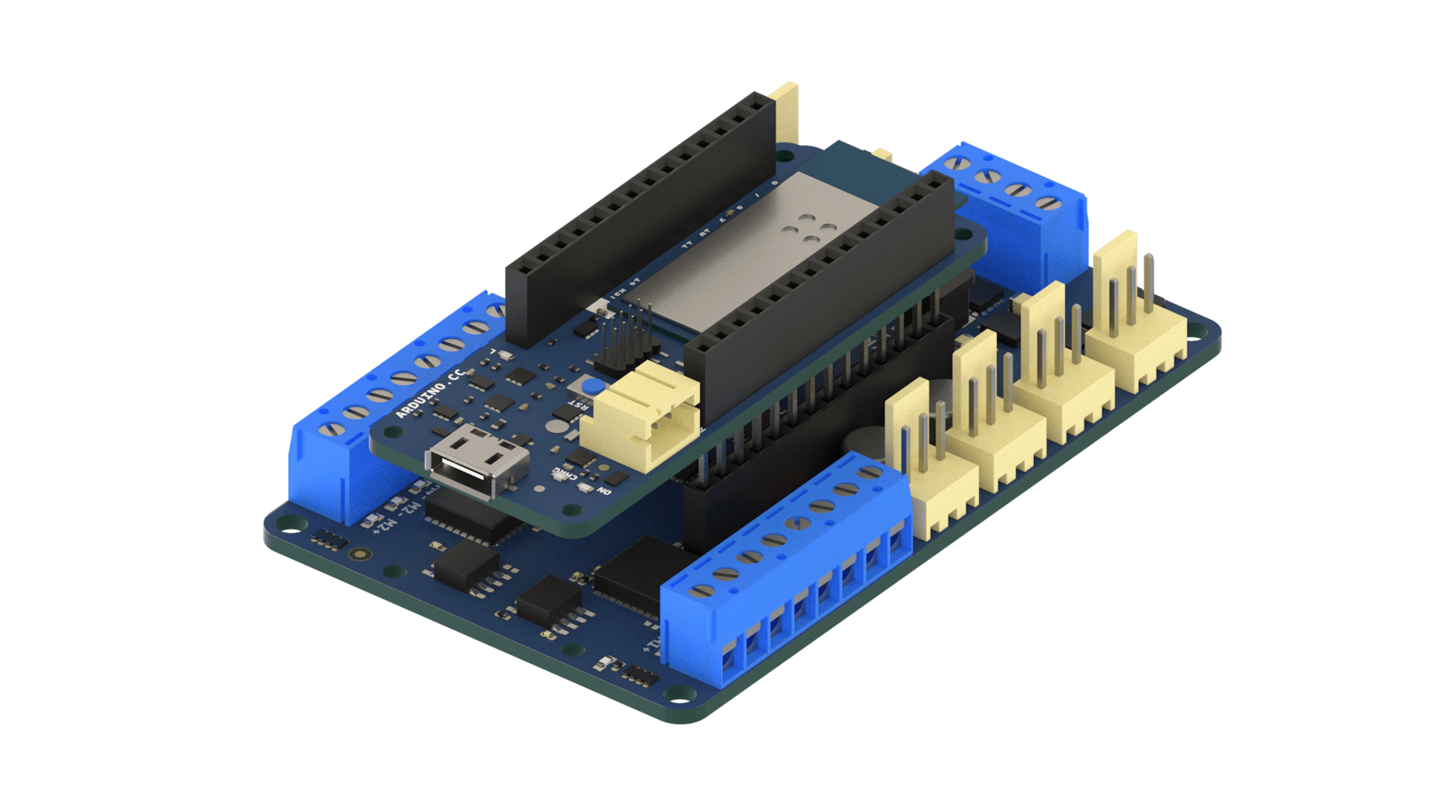
ARDUINO MKR MOTOR CARRIER
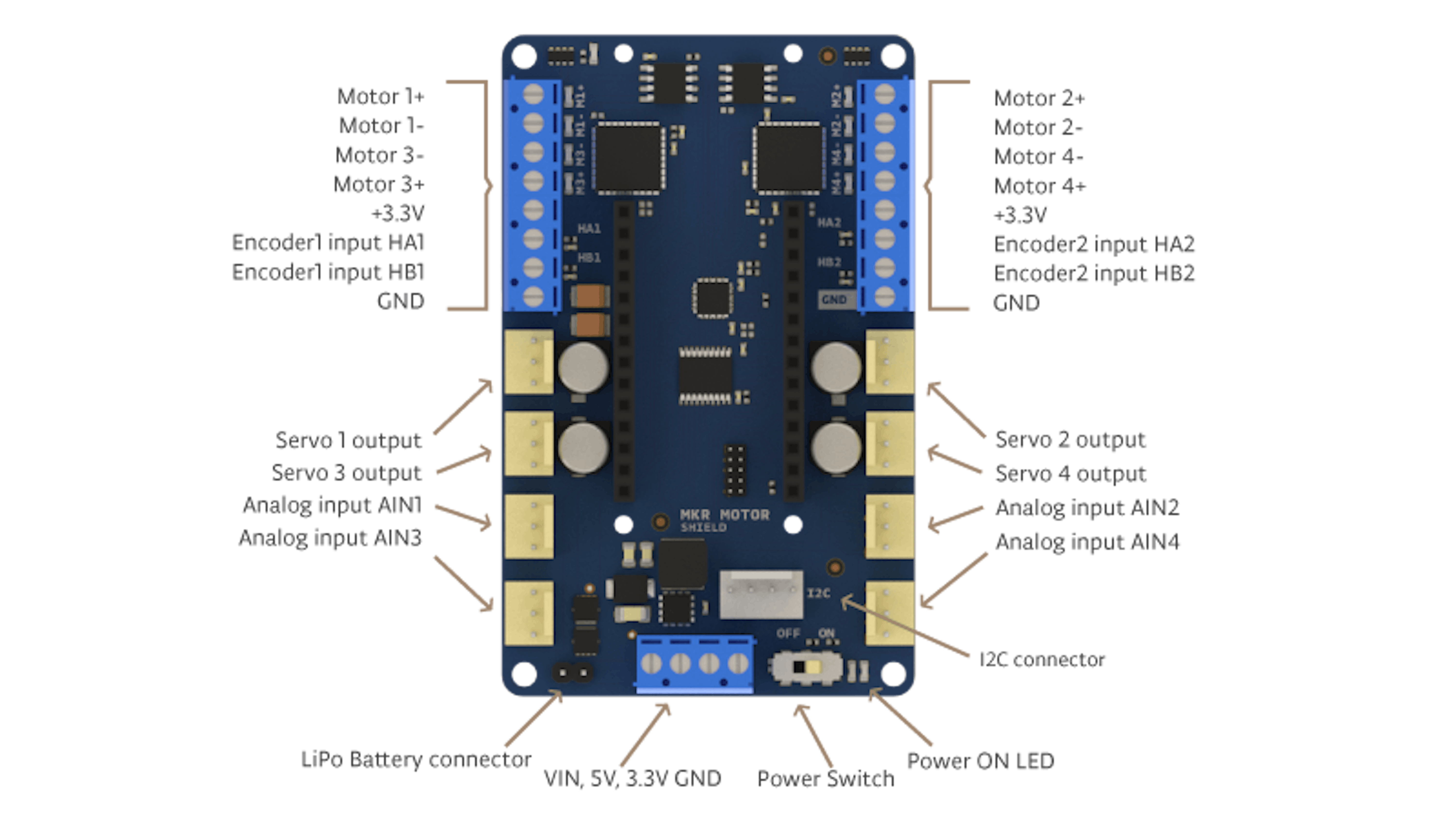
The MKR Motor Carrier (also known as MKR motor carrier board) is an MKR add-on board designed to control servo, DC, and stepper motors. The Carrier can also be used to connect other actuators and sensors via a series of 3-pin male headers.
The summary of features is shown below:
- Compatible with all the boards in the MKR family
- Four simultaneous servo motor outputs
- Up to four simultaneous DC motors (two high performance + two standard performance)
- Two simultaneous stepper motors (alternative to the DC motors)
- Sensing of current feedback for the high-performance motors
- Two inputs for encoder sensors
- Four inputs for analog sensors (3-pin compatible)
- Possibility to read the status of the batteries
- ON-OFF switch with Power ON LED
- LiPo battery connector (2S or 3S compatible) and power terminal block for alternative power source
- LEDs to visually indicate the direction of the rotation of the DC motors
- On-board processor for automated control of some of the outputs
- I2C connector as a 4-pin male header
The MKR Motor Carrier features two MC33926 motor drivers for high-performance DC motor control with direct connection to the MKR1000, current feedback, and capacity for up to 5 Amps (peak). In addition, there are two DRV8871 drivers that are controlled from a SAMD11 microcontroller that communicates with the MKR1000 via I2C (SPI optional). The SAMD11 is also used to control the servos, read the encoders, and read the battery voltage. There is an interrupt line connecting the SAMD11 (on PA27) and the MKR board.
Electrical characteristics:
- Reverse current protection in the power pins
- Max current MC33926: 5 Amps Peak, RMS current depending on the degree of heatsink provided
- Max current DRV8871: 3 Amps peak, current limited by current sense resistor
- Rated voltage: 6.5V to 20V
Note that for extended use or high-current motors, an extra heatsink (and eventually a fan) might be required for the drivers. For the examples and projects included in this kit, it is not needed. There will be specific explanations provided at different points in the documentation regarding how to safely operate the Carrier, not following them will put the Carrier, the motors, and eventually the MKR1000 at risk.
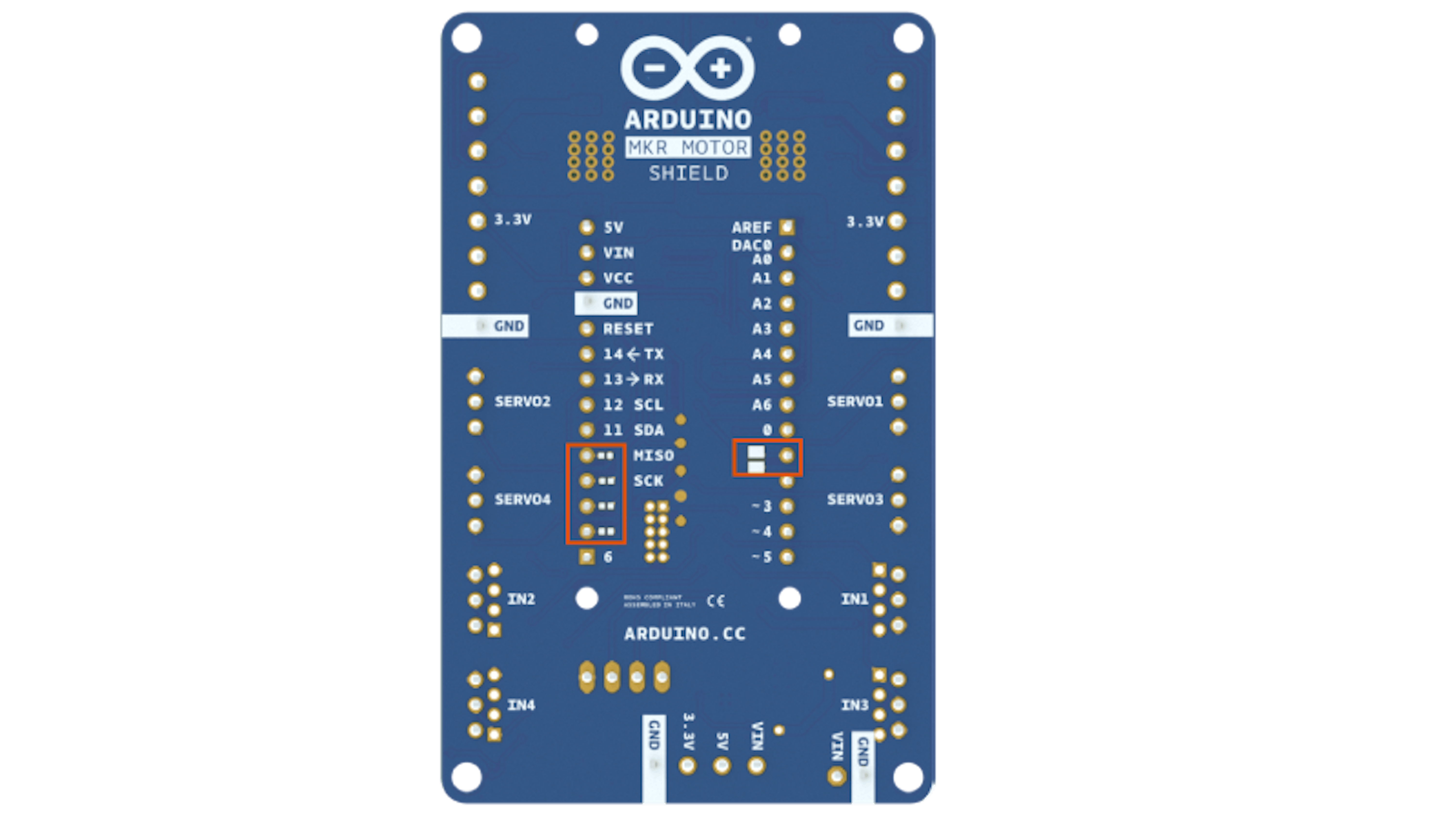
When plugging the MKR1000 and the Motor Carrier, some of the pins will stop being available for you to use in your code, as they will be needed to control some of the features of the Carrier. For example, the current feedback from the two MC33926 drivers is connected directly to some of the analog pins on the MKR1000. The following list explains which pins of the MKR1000 are used to control the Carrier:
- Analog pin A3 for current feedback from Motor3
- Analog pin A4 for current feedback from Motor4
- Digital pin D2 for IN2 signal for Motor3
- Digital pin D3 for IN1 signal for Motor3
- Digital pin D4 for IN2 signal for Motor4
- Digital pin D5 for IN1 signal for Motor4
- Digital pin D6 for Interrupt signal from the SAMD11 to the MKR1000
- Digital pin D11 for the SDA signal (I2C)
- Digital pin D12 for the SCL signal (I2C)
Also, some pins can optionally be connected via a soldering jumper or a 0 Ohm resistor. These pins are:
- Digital pin D1 for the SF signal from the MC33926 drivers (optional)
- Digital pin D7 for the SPI SS signal (optional)
- Digital pin D8 for the SPI MOSI signal (optional)
- Digital pin D9 for the SPI SCK signal (optional)
- Digital pin D10 for the SPI MISO signal (optional)
To use the Carrier, you will need to plug an MKR board (the MKR1000, MKR Zero, or other) on the headers at the center of the board. Make sure the MKR board is connected in the proper direction. You can do this by making sure the info printed on the side of the headers are matching for both the MKR board and the Motor Carrier.
Once the board is properly connected to the Motor Carrier, you can start programming the board. To control the motors, you will need to import the MKR Motor Carrier library. You can find more information about the library here. If you want to read more about how to install a library, follow this link.
When working with motors, you will need an external source to feed the motor drivers and power up the motors. You can do this by connecting a LiPo Battery to the battery connector or using an external power source and connecting it to the VIN input on the terminal block. It is recommended to do these operations with the power switch at the OFF position. Once the external power is connected to the board, the power switch can be turned on.
In the projects of this kit, we will be using the Motor Carrier with an MKR1000 because of the Wi-Fi capabilities of that board. Thanks to a special configuration within MATLAB, the board can communicate directly to the software as long as they are on the same wireless network.
The Motor Carrier will be used in the three projects:
- Self-Balancing Motorcycle: In the self-balancing motorcycle, the Carrier will be used to control the inertia wheel in the center of the motorcycle. It will also command the geared DC motor in the back wheel to move forward or backward, and a servo in the front to steer the motorcycle. The ultrasonicund range sensor and the hall sensor will be connected to the carrier as well, using some of the 3-pin connectors. The Hall-effect sensor will be used to limit the speed of the inertia wheel, while the ultrasonicund range sensor is required to stop the motorcycle from crashing into any objects when moving forward.
- Mobile Rover: In the rover, the MKR Motor Carrier will be used to control the two DC geared motors and the encoders that are connected to the rover's wheels. In addition, the Carrier will be used to control a servo motor in the front of the vehicle, providing the rover with a lifting mechanism. An ultrasonicound range sensor will also be connected to the Carrier for obstacle avoidance.
- Drawing Robot: In the drawing robot, the Carrier will be used to control the two DC geared motors with encoder to locate the robot on the whiteboard. In addition, it will be used to control a servo motor involved in changing the marker color as well.
Read more about the MKR Motor Carrier at the Arduino store, where you will find documentation about the design, datasheets, and other materials.
MOVING A DC MOTOR WITH ARDUINO
To introduce you to MATLAB, Simulink, and the Arduino support packages, you will complete a short project in Sections 2.2 and 2.3 that uses both MATLAB and Simulink to target the Arduino board and some of the peripheral devices included in the Arduino Engineering Kit. In this short project, your objective is to determine the relationship between the rotational speed of a DC motor and the applied voltage. You will learn how to use that relationship to develop a speed control application that you will upload to the Arduino MKR1000 board. You will use a rotary encoder to measure the angular displacement of the motor from a reference angle, and use successive angle measurements to calculate the motor speed. To learn more about encoders, see 3.3 Encoders in Chapter 3 .
The above-mentioned project will unfold in the following sections, and will teach you how to:
- Navigate the MATLAB user interface,.
- Enter MATLAB commands,.
- Create, access, and modify data,.
- Perform calculations with data,.
- Visualize data,.
- Write scripts and functions and.
- Create and simulate a Simulink model.
2.2
Matlab getting started
MATLAB is powerful software that allows you to make complex calculations on large datasets. MATLAB has its own textual programming language with instructions that can be collected into scripts. You could imagine MATLAB to be like a command-line interface for mathematical operations: you can execute commands directly on a terminal-like interface or make batch scripts that can be invoked from the same terminal.
With MATLAB, you can take sets of images and apply different types of filters on them to plot histograms, multiply large matrices of data, or create dialogues to input data manually. You can also communicate with Arduino boards as a way to bring live sensor information into your programs or control actuators plugged to the board.
INSTALL MATLAB (AND SIMULINK)
As this kit aims to introduce concepts in a very empirical way, we will quickly get hands-on with both hardware and software. In the previous section, we explained how to install Arduino separately and to use it in a couple of simple examples where you had to type your code.
MATLAB and Simulink enable a different way of programming Arduino boards using a visual programming language (VPL for short), as we will show you in the following sections. Note: Arduino is installed as a plugin to MATLAB. This means that even if you installed it before, you must install it again whenever you add the Arduino-related tools to your MATLAB installation.
Install MATLAB, Simulink, and any other extensions you will need. You can find more information about how to do that in "1.3 Tools" and registering using the codes provided with this kit. Use your official MATLAB registration codes whenever you install the software. Once you have installed the programs, you will be ready to try the examples presented in the rest of this chapter.
WORKING WITH DATA IN MATLAB
In this section, you will learn:
- How to identify the core components of the MATLAB desktop environment,.
- How to issue MATLAB commands in the command window,.
- How to create scalar and vector variables and apply functions and arithmetic operations to existing variables,.
- How to access and manipulate data stored in vectors,.
- How to create and label line plots of vector data and.
- How to save and load MATLAB data to and from disk.
Let's start by getting familiar with the MATLAB environment. In this section, you will use the MATLAB Command window to learn some of the MATLAB language syntax, how to create, modify, and analyze MATLAB variables, and how to generate informative visualizations of your data. Eventually, you will use the techniques in this section to develop input test cases for Arduino and analyze and visualize the output from Arduino peripheral devices
NAVIGATING THE MATLAB DESKTOP
Launch MATLAB from your Start menu or by double-clicking the executable file. For Windows users, the executable is called matlab.exe and is usually located in C:\Program Files\MATLAB\R2018a\bin where 2018a indicates the version number of the software in use. Note: This kit is aimed at MATLAB version 2018a or newer.
Once you have launched the MATLAB Desktop, you will notice four panels in the MATLAB Desktop that you should familiarize yourself with. They are named Current Folder, Command Window, Workspace, and Toolstrip.
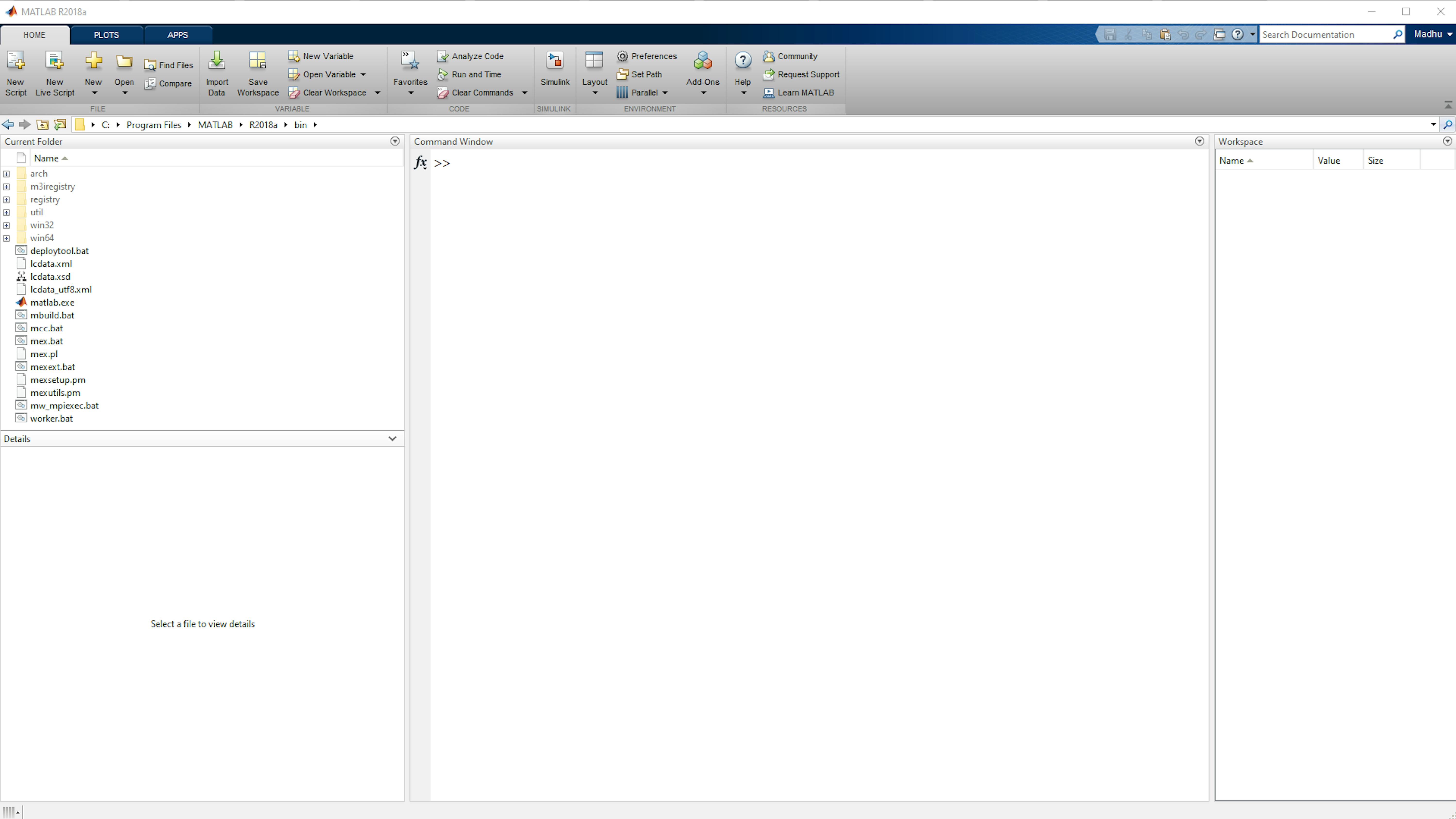
On the left, the Current Folder panel acts just like your file explorer: it indicates your current location in the computer's file structure and its contents. The Command Window is the command-line interface (CLI for short) where you can experiment with commands in the MATLAB language before adding them to a MATLAB program. The Workspace will display a list of existing MATLAB variables and some of their properties. At the top of the MATLAB desktop is the colorful Toolstrip, which contains buttons for basic file operations, basic MATLAB operations, and software environment settings.
Just below the Toolstrip, you will see a horizontal white bar that indicates the current location within your file system. It is important to be mindful of your current folder (the folder from which you are executing MATLAB commands), because various operations in MATLAB and Simulink will generate files into the current folder. It is useful to have a designated "work" directory, to save your work into and keep all generated files in one place.
Navigate to the "work" folder by typing the following command in the MATLAB Command Window and pressing Enter.
>> cd(arduinokit.workRoot)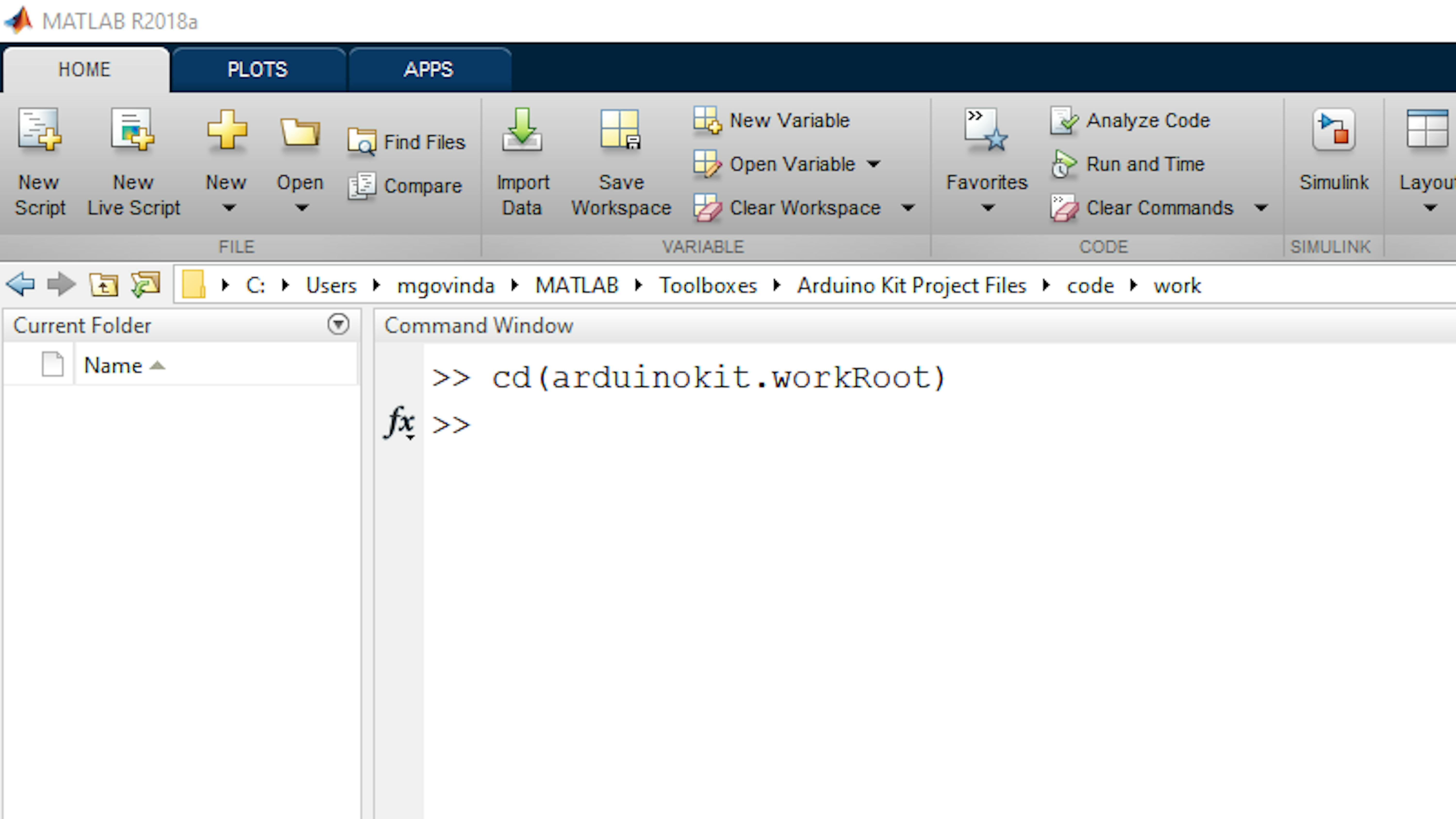
ENTERING MATLAB COMMANDS
Let's now get used to some basic MATLAB syntax. In the Command Window, type the following command to create a new variable a;
>> a=7Next, create a variable called b by assigning a value to it.
>> b = 8;You can revisit previous commands by using the UP button on your keyboard. Press the UP key until you get back to your original command, a=7, and press Enter. Now bring the same command back, but change the variable name to c. These operations will generate three variables ( a, b, and c) that will be available for you to use. It is now possible to make operations using the variables as part of equations, vector declarations, etc.
As you can see, white space around operators is irrelevant in terms of MATLAB execution, but it is often easier to read code in which operators and operands are spaced out.
If you want to simply execute a line of code without seeing the result in the Command Window, you can end the line with a semicolon (;).
VARIABLES AND VECTORS
Look in the Workspace panel. You will see there the three MATLAB variables a, b, and c. By default, the Value of each variable is shown, provided it is not too large to be displayed in the Workspace panel. You can display various other attributes of your variables by right-clicking the column headers in the Workspace panel.
Right-click the column headers, which will display a series of options in a list; locate the Size column and click to enable it. This will add a new column to the interface that shows the sizes of the variables.

In MATLAB, the size of a variable indicates its dimensions, in a rows x columns format. As you can see, all your current variables are 1 x 1, or scalars. Let's create another scalar. Type the following command, and then examine the Workspace:
>> A = 1.23;You can see that the variables A and a are distinct in MATLAB. In other words, MATLAB is a case-sensitive language. Try the following commands, but this time do not peek at the Workspace yet:
>> B = 4.56;
>> A = B;
>> B = 3.14;
What do you think the value of A is? Check the Workspace to see if you were correct.
The correct answer is that the value of A is 4.56. As you can see, MATLAB variables only store values. They do not propagate relationships with other variables that may have been used originally. If you would like A to reflect the new value of B, re-enter the command A=B.
Now let's delete some variables. The clear command deletes a subset or all the variables from the Workspace. Delete the variables a and b by typing the following command, and then examine the Workspace:
>> clear a bYou can delete all the variables by typing the following command:
>> clearVECTORS
While we can achieve a lot with scalars, most meaningful data consists of a 1-dimensional array of numbers, called a vector. A vector can be oriented as a row vector or a column vector. Create a row vector v1 of length 7 by entering the following command, and then examine your Workspace:
>> v1 = [1 3 2 6 4 4 9]
Now create a column vector v2 of length 5 as follows, and examine your Workspace:
>> v2 = [2;5;7;1;2]When you have variables that are larger than a scalar, you may need to access a subset of that variable. This is known as indexing. Enter the following commands to index into a 1x1 portion of vector variables v1 and v2:
>> x = v1(3)
>> x = v2(5)
>> x = v2(end)
Similarly, you can use variable indexing to modify a portion of an existing non-scalar variable. Enter the following command to change one value in v2:
>> v2(2) = -1You can reorient a vector as a column or row using the transpose operator ('). Enter the following command to reorient v2 as a row vector:
>> v2 = v2'Earlier you used square brackets ([ ]) with comma ( , ) or semicolon ( ; ) delimiters to create row and column vectors respectively. This syntax is useful to create short vectors with arbitrary values. What about much longer vectors? Often you will need a vector of uniformly spaced values to represent a series of periodic time values or a geometric coordinate. Other long vectors might be populated by a series of sensor values measured at those times or coordinates. Still other vectors might be the result of some processing of the raw measurements. For now, let's just generate vectors of uniformly spaced values. Try the following commands:
>> v3 = 0:6
>> v4 = 0:0.5:6
Now let's create a vector with some real-world relevance:
>> v4 = (0:0.5:6)'The vector theta will represent an angle expressed in radians, spanning two full revolutions. We will use this vector in the following sub-section.
>> theta = -2*pi:pi/10:2*pi;BUILT-IN FUNCTIONS
MATLAB comes with a vast library of built-in utilities, called functions, which can operate on your data to produce meaningful results. Try the sin function, using the following syntax:
>> y = sin(pi/2)The sin function, and the other built-in trigonometric functions, operate on angles expressed in 3radians. Now try taking the sine of many angles at once, and then examine y in your Workspace:
>> y = sin(theta);When you input a vector into a function, and the output is a vector of the same size, the function is said to be vectorized. Vectorization is a key feature of the MATLAB language, and it allows you to write simple, concise lines of code that execute many operations at once, and which closely resemble mathematical expressions. You can input multiple operations and function calls in a single line of MATLAB code. Enter the following statement to apply a phase offset, a frequency scaling, a gain, and an amplitude bias to the sine wave:
>> y = 3*sin(2*theta + pi/2) - 1.5;MATLAB has many built-in functions that generate outputs of arbitrary dimensions. Sometimes it is useful to produce an array of a given size that you will later populate with meaningful data. Try the following commands to generate two-dimensional matrices of all ones and all zeros:
>> z = ones(3,4)
>> z = zeros(4,3)
Since a given MATLAB expression can operate under many different circumstances, you may need to determine certain properties of your data before operating on it. Use the following commands to determine the size of y, z, and theta:
>> size(y)
>> size(z)
>> size(theta)
Now let's use this information to allocate an array a that is the same size as theta:
>> a = zeros(size(theta));Another function that operates similarly to zeros and ones is randn, which generates an array of normally distributed random numbers with a mean of zero and standard deviation of 1. Try generating a list of 20 such numbers by calling the following function:
>> randn(20,1)Finally, combine the previous techniques to add some random noise to your sine wave to produce a new vector z:
>> z = y + 0.3*randn(size(theta));VISUALIZING DATA
The quickest way to gain insight from your data is to visualize it using some type of plot. In this introduction you will create simple line plots of your vector data. Use the following command to visualize the values in the vector y:
>> plot(y)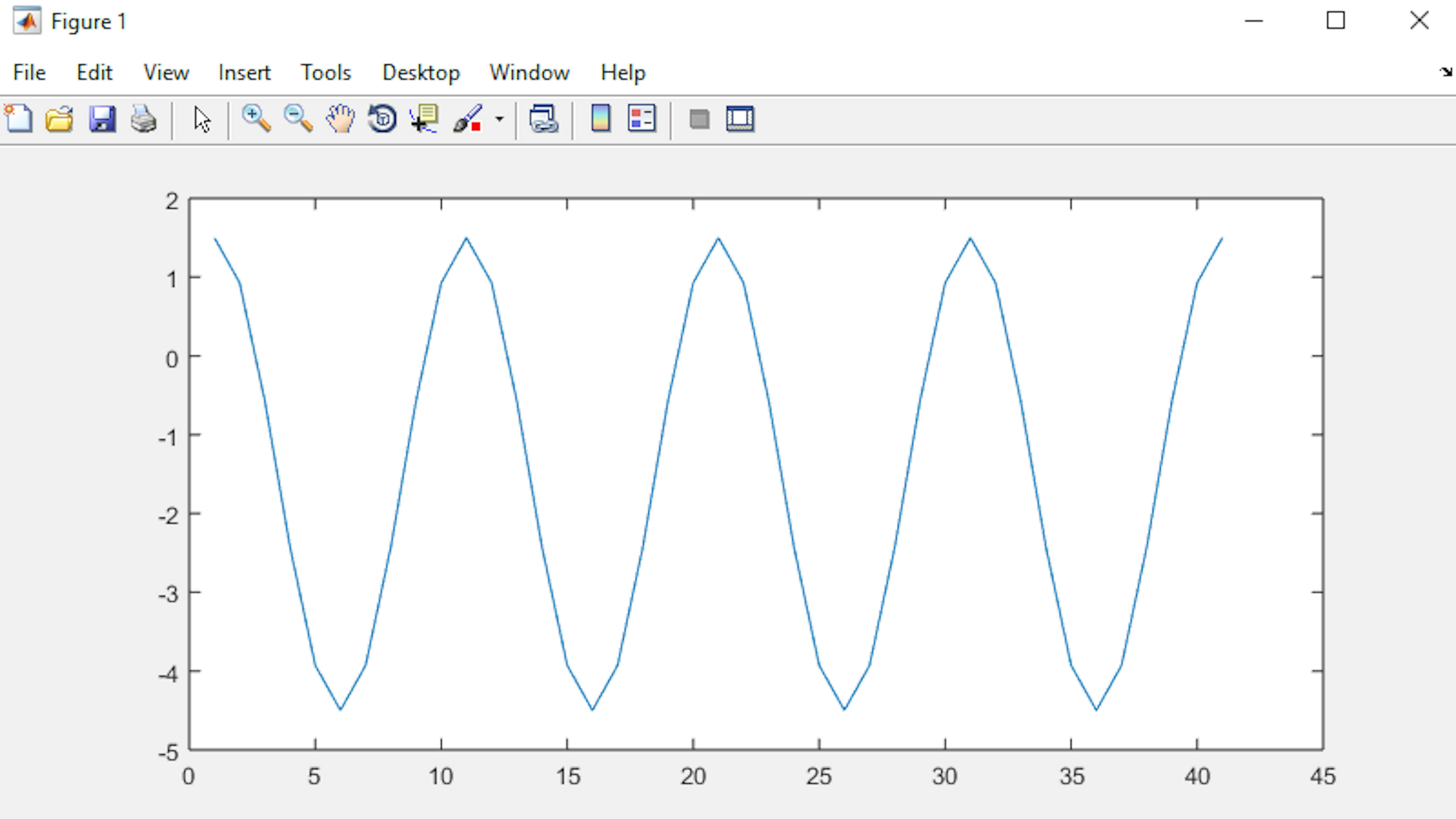
As you can see, when you plot a single vector, it renders as a continuous line joining the discrete values in that vector. The x-axis represents the indices of that vector from 1 to N. Now let's plot the vector y against a more meaningful variable, the angle theta in this case;
>> plot(theta,y)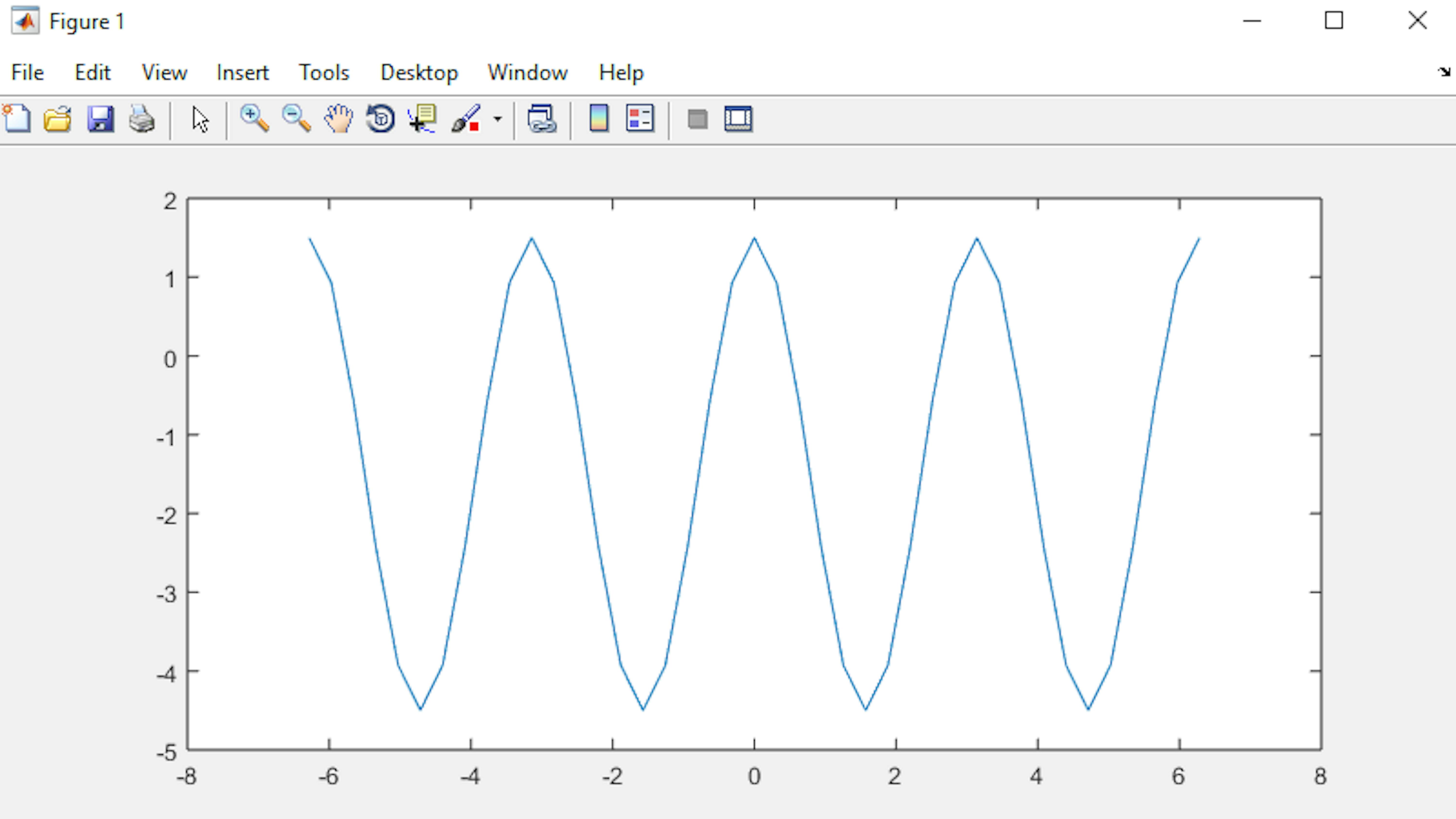
When you input two vectors to the plot function, the corresponding ordered pairs are plotted and connected by straight lines. Also notice that the new plot overwrote the old plot. Suppose you want to keep a plot in the figure window but plot a new line on top of it. You must hold the plot to avoid overwriting it. Try the following commands to plot a new line (taken from the variable z) on top of the sine wave:
>> hold on
>> plot(theta,z)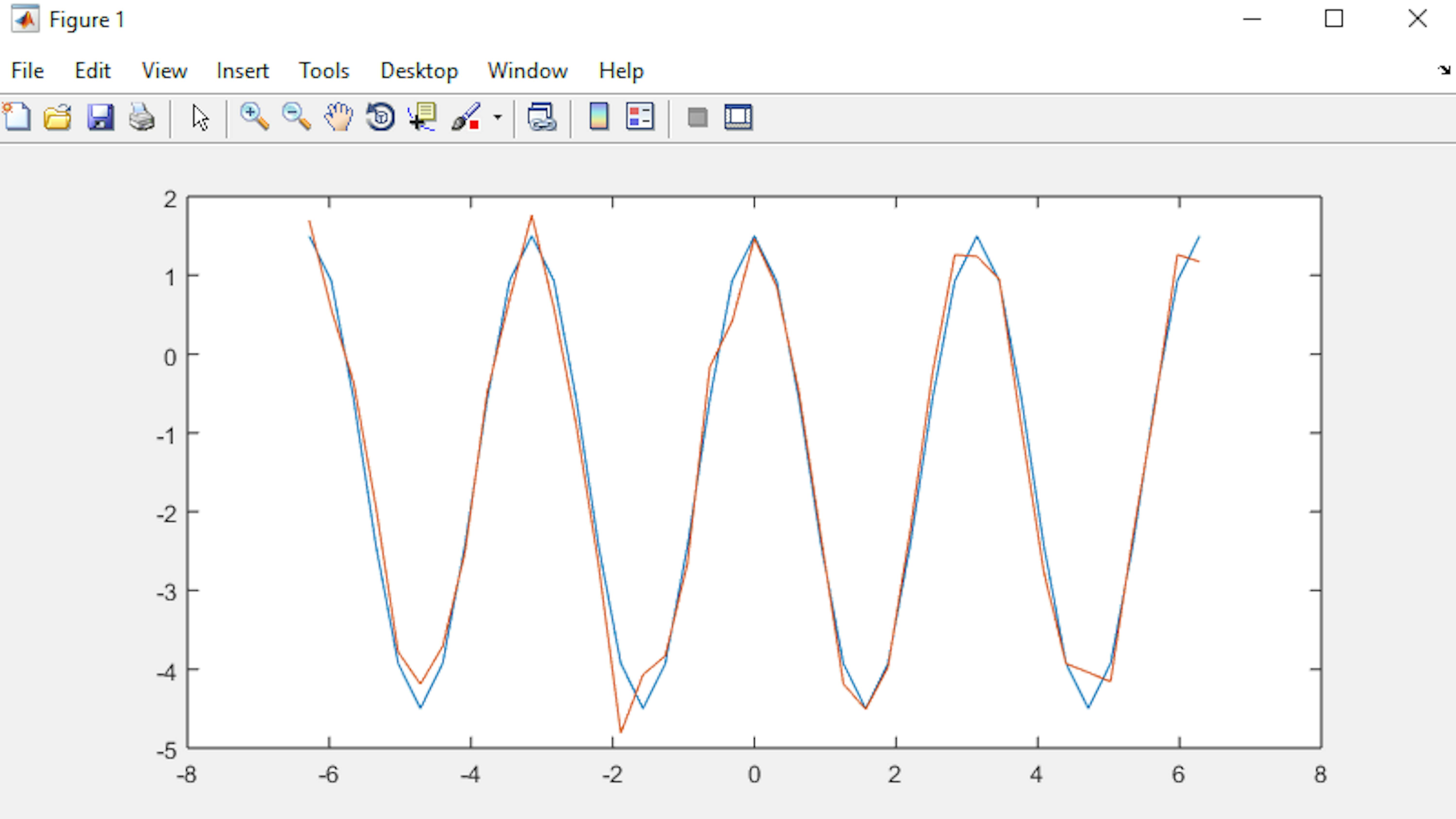
Finally, let's add some labels to the figure so that it is easier for your audience to understand. Use the following commands to add axis labels, a title, and a legend to distinguish the two lines:
>> xlabel('Phase (radians)')
>> ylabel('Amplitude')
>> title('Ideal vs. Noisy Oscillations')
>> legend('Ideal','Noisy')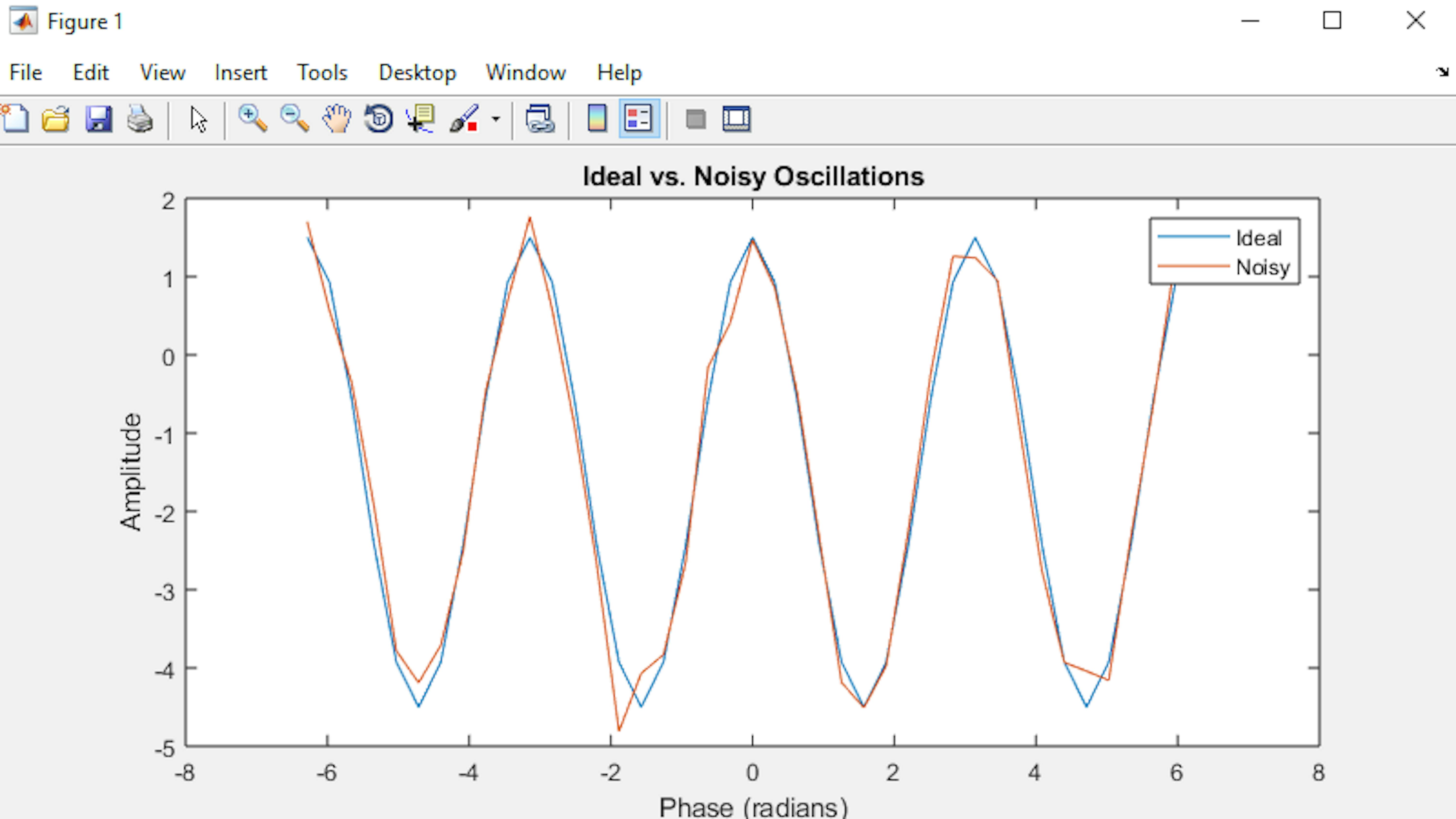
Note how the function legend works, as it assigns the labels to the plotted lines in the same order they were drawn.
SAVING AND LOADING DATA
You now have several variables in your workspace. Suppose you need to call it a day and shut down MATLAB. When you exit MATLAB, all your workspace data will be deleted. You can save important data to disk. Use the following command to save the variables theta, a, y, and z:
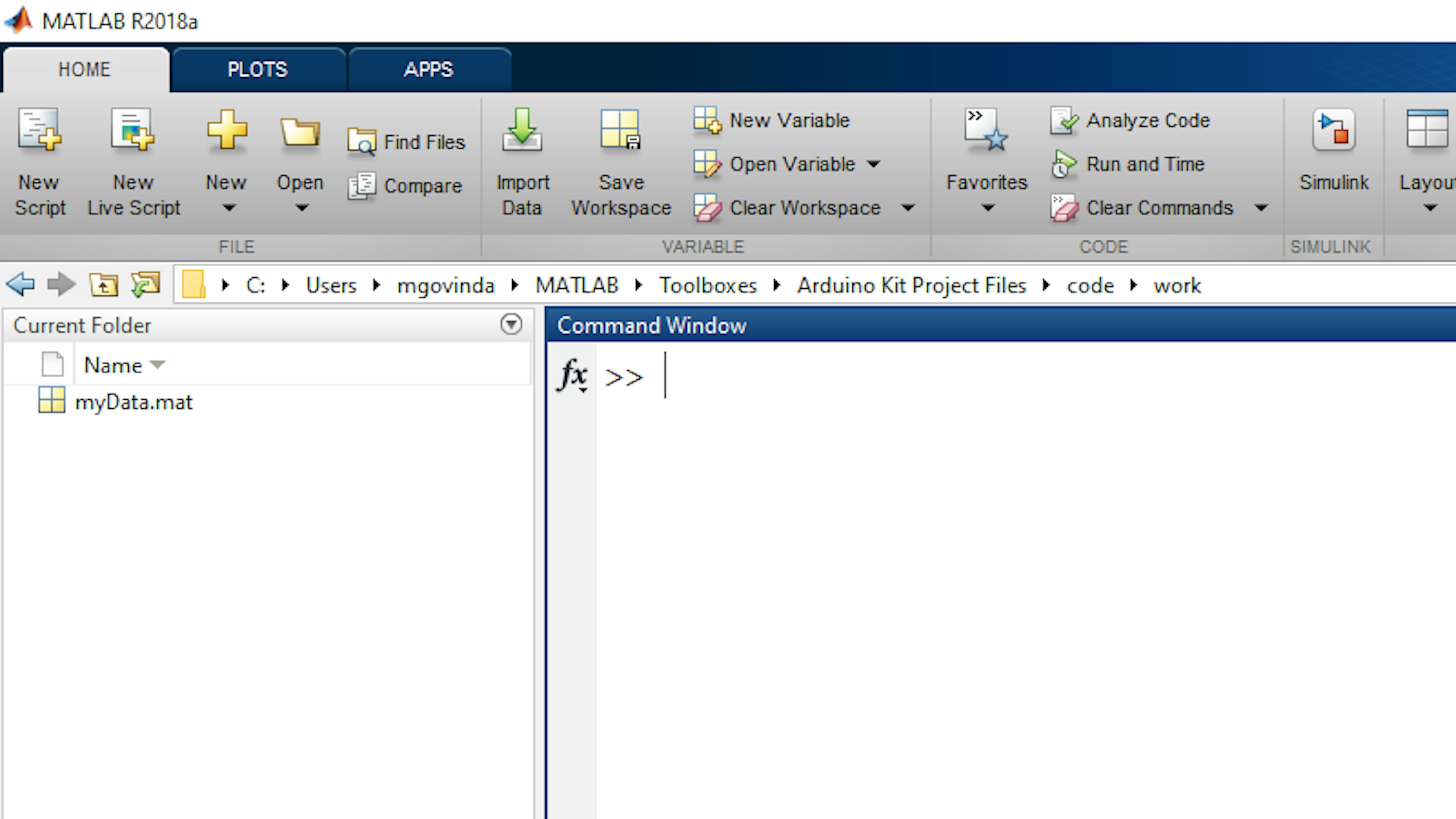
>> save myData theta a y zNow, examine the Current Folder panel in the MATLAB desktop. You will see that MATLAB has created a new file called myData.mat:
Let's test your new MAT-File. Use the following commands to clear all variables from the Workspace and then reload them using the load command:
You will see now that the Workspace only contains the previously mentioned list of four variables and that all the others are gone.
>> clear
>> load myData
COMMUNICATING WITH ARDUINO AND EXTERNAL DEVICES IN MATLAB
In the previous section, you learned about types of variables that can be used in MATLAB, how to use functions, and how to visualize data. The next step is learning how to get your Arduino board to connect to MATLAB and learning enough of the basics to feel comfortable using the software on your own.
In this section, you will learn:
- How to identify the native pin functionalities on the Arduino MKR1000.
- How to identify the functionalities on the MKR1000 Motor Carrier.
- About pulse width modulation (PWM) signal structure, and how it is used to drive a DC motor and other devices.
- About the mechanism by which a rotary encoder measures rotational angle.
- How to connect MATLAB to Arduino MKR1000.
- How to configure and manipulate digital pins on Arduino MKR1000.
- How to configure and drive a DC motor from MATLAB.
- How to configure, read, and process data from a rotary encoder in MATLAB.
In this section, you will use the MATLAB Support Package for Arduino to access the Arduino MKR1000 board and two of the external devices that come in the Arduino Engineering Kit: the 100:1 Gearhead DC Motor and the Magnetic Encoder, which comes already connected to the motor's drive shaft. From the MATLAB environment, you will learn how to drive the motor at specific voltages and sense the rotational motion of the motor through the rotary encoder.
CONFIGURING ARDUINO LIBRARIES
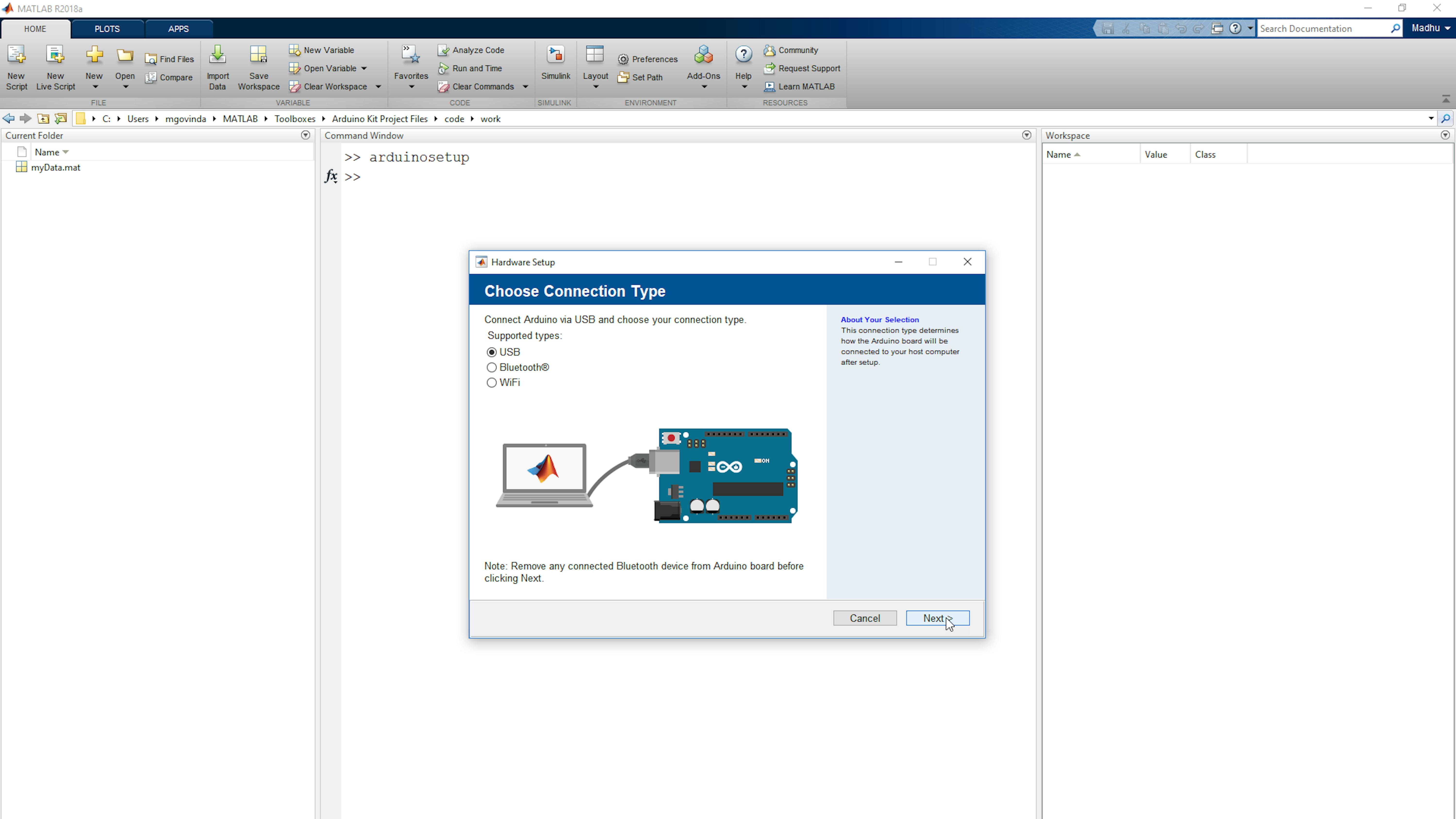
Next, you will set up the MKR1000 board in MATLAB. Type the following command to start:
>> arduinosetupThis will open the Hardware Setup window. For most of this lesson, you will communicate between your computer and the MKR1000 board via USB connection. Therefore, you should select USB from the available options and click Next.
Next, you will select your Arduino board type, the port through which you will communicate with it, and the external devices you will need have access to. For this example, you will need to access to the MKR Motor Carrier, which is a board that interfaces the MKR1000 with up to four DC motors, up to two rotary encoders, and up to four servo motors, as explained earlier. In this example we will use one DC motor and one rotary encoder.
I2C is a digital communication protocol that enables one device to transmit data to and from several other devices. When the MKR1000 drives DC motors through this Carrier, it can send the motor drive command using I2C communication (two of the DC motors are connected to a driver that goes directly to the MKR board, while the other two are controlled from a processor located on the Carrier). Similarly, the rotary encoders send angular position data back to the MKR1000 board via I2C. By selecting I2C, you are loading the appropriate resources to the MKR1000 board to enable such communication.
Set your board to MKR1000. Set your communication port to the COM or ttyACM or usbmodem (depending on the OS) port you found earlier. Select Arduino/MKRMotorCarrier and RotaryEncoder. Click Program.

Note: This may take several minutes. If you receive an error message related to source not being found for the Arduino/MKRMotorCarrier library, then type edit ArduinoKitHardwareSupportReadMe.txt in MATLAB Command Window and follow the instructions provided on this text file.
After the libraries have successfully loaded to the MKR1000 board, click Next and complete the remainder of the dialog. You are uploading firmware to the MKR board that will enable it to communicate back to your computer, where MATLAB will be executing commands with the help of the information that will be captured by sensors and sending it back to actuators via the same communication channel.
CONNECTING MATLAB TO ARDUINO
Now that the required resources have been loaded onto the MKR1000 board, we can access MKR1000 and the devices from MATLAB. Enter the commands below to clear your Workspace and create an "arduino" object:
>> clear
>> a = arduino
Unlike the variables in the previous section (which were numeric scalars, vectors, and matrices), the new variable a is a MATLAB object of type arduino. MATLAB objects are specialized variables with a fixed set of properties, which are meaningful values stored within the object, and methods, which are functions that operate on objects of that type. We will access and invoke some of these properties and methods shortly. While the Arduino object (or any derived object) exists in your Workspace, MATLAB is connected to the Arduino board via a server utility. If you want to release this MATLAB server from Arduino so that you can run some other program on Arduino (for instance, from the Arduino software or Simulink), you need to delete the Arduino object in MATLAB. Enter the following commands to release Arduino from MATLAB and then re-establish the connection:
>> clear a
>> a = arduino
MKR MOTOR CARRIER AND DC MOTOR
Next you need to access the MKR Motor Carrier so that you can use the DC motor and rotary encoder. In this section, it is assumed that you have not yet assembled the parts from the kit into any of the projects. If you have a pre-built project, a) Drawing Robot, b) Mobile Rover or c) Self Balancing Motorcycle, please take precautionary measures. For example, place the rover on top of a pedestal and ensure that the wheels can spin freely while running the motor and encoder experiments in the next two sections.
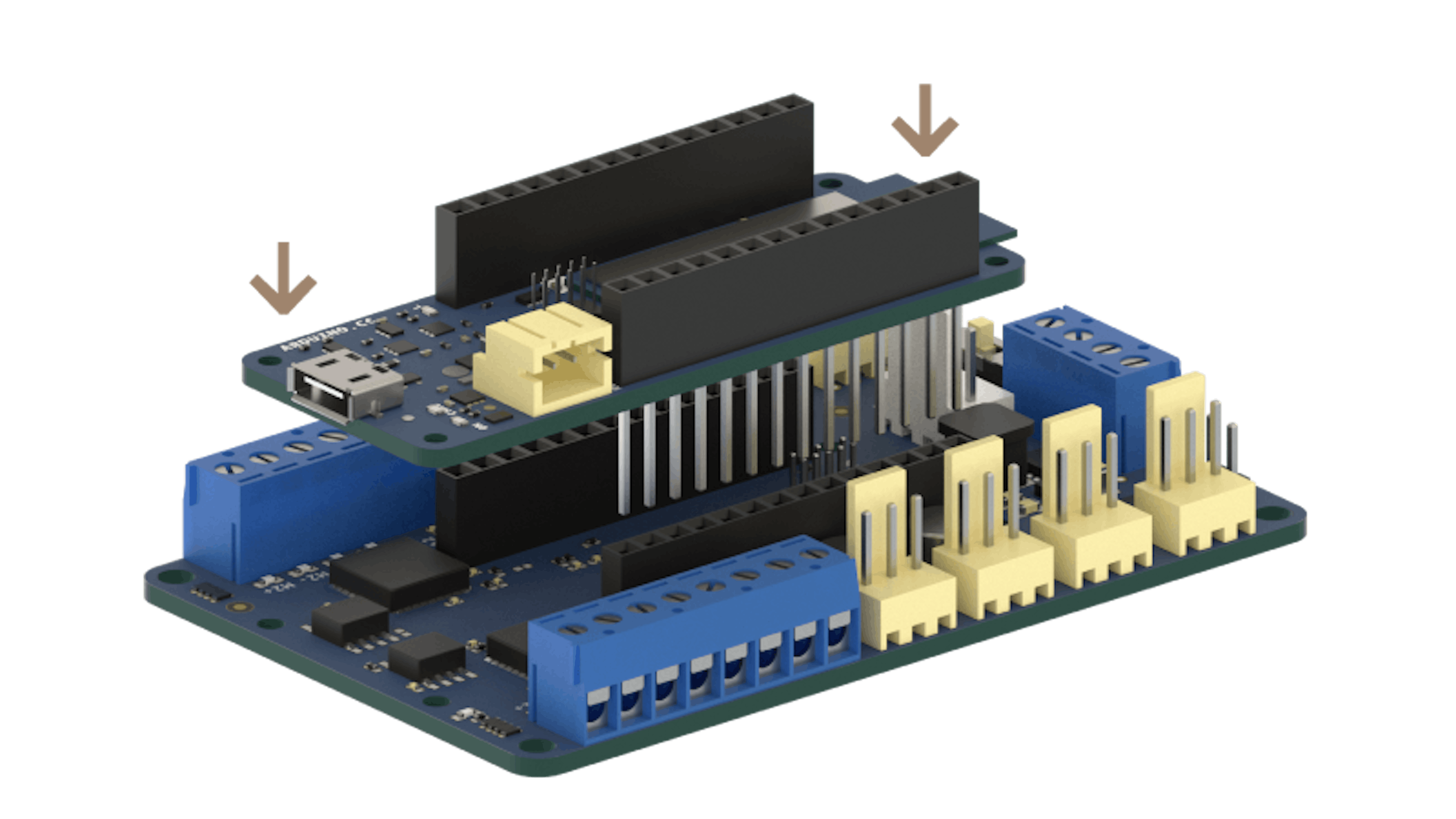
Disconnect the USB cable between MKR1000 and your computer, ensure that the Motor Carrier's switch is in OFF position and then attach the Motor Carrier to the MKR1000 board. You can do this by aligning the corresponding pin labels and pressing down on the MKR1000 board firmly. It is strongly recommended that to perform any operation of mounting or removing parts from a circuit, you always disconnect them from both power sources (battery and the USB cable).
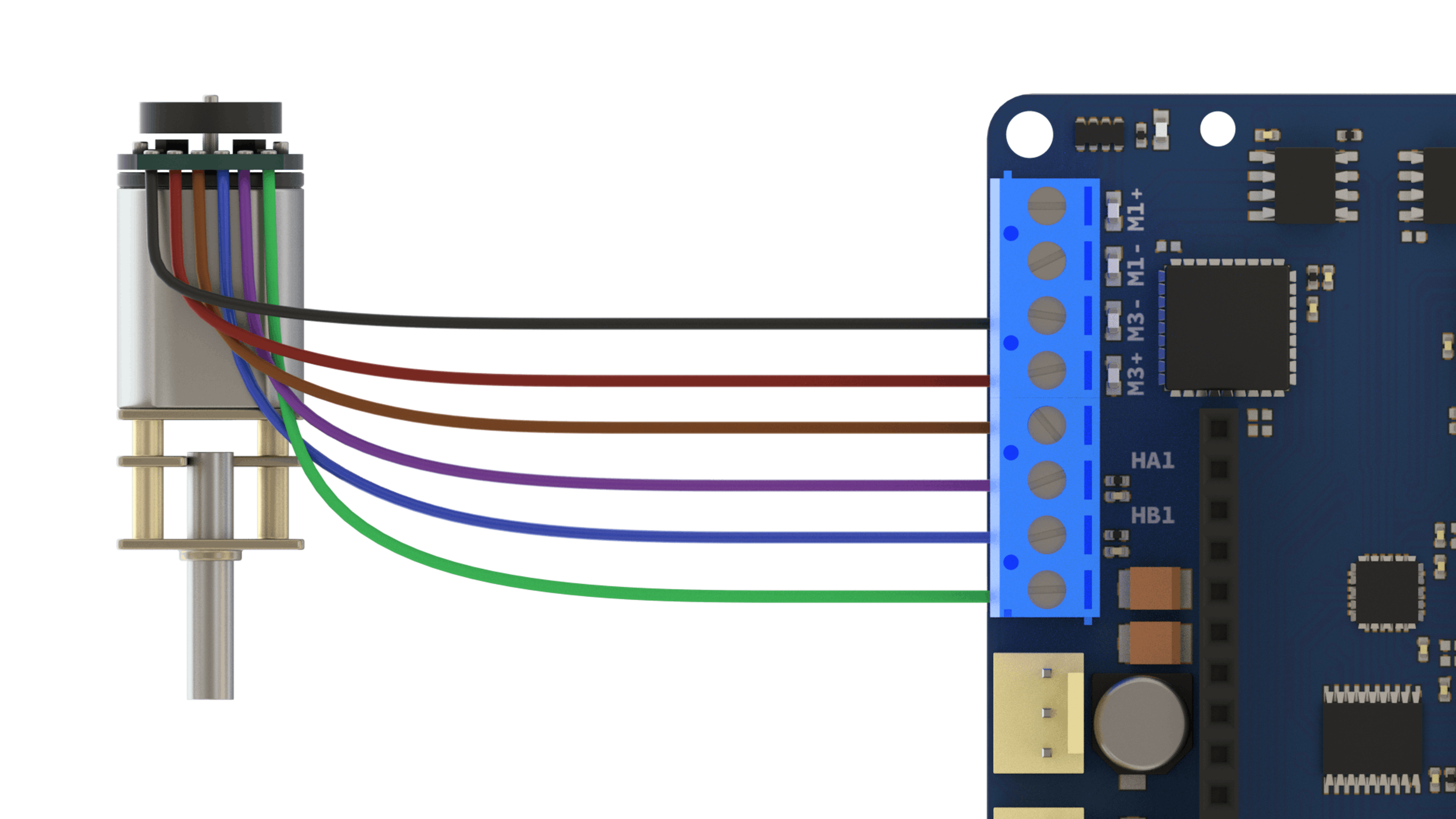
Now let's set up the DC 100:1 gearhead motor. First, let's examine the wires coming out of the motor.

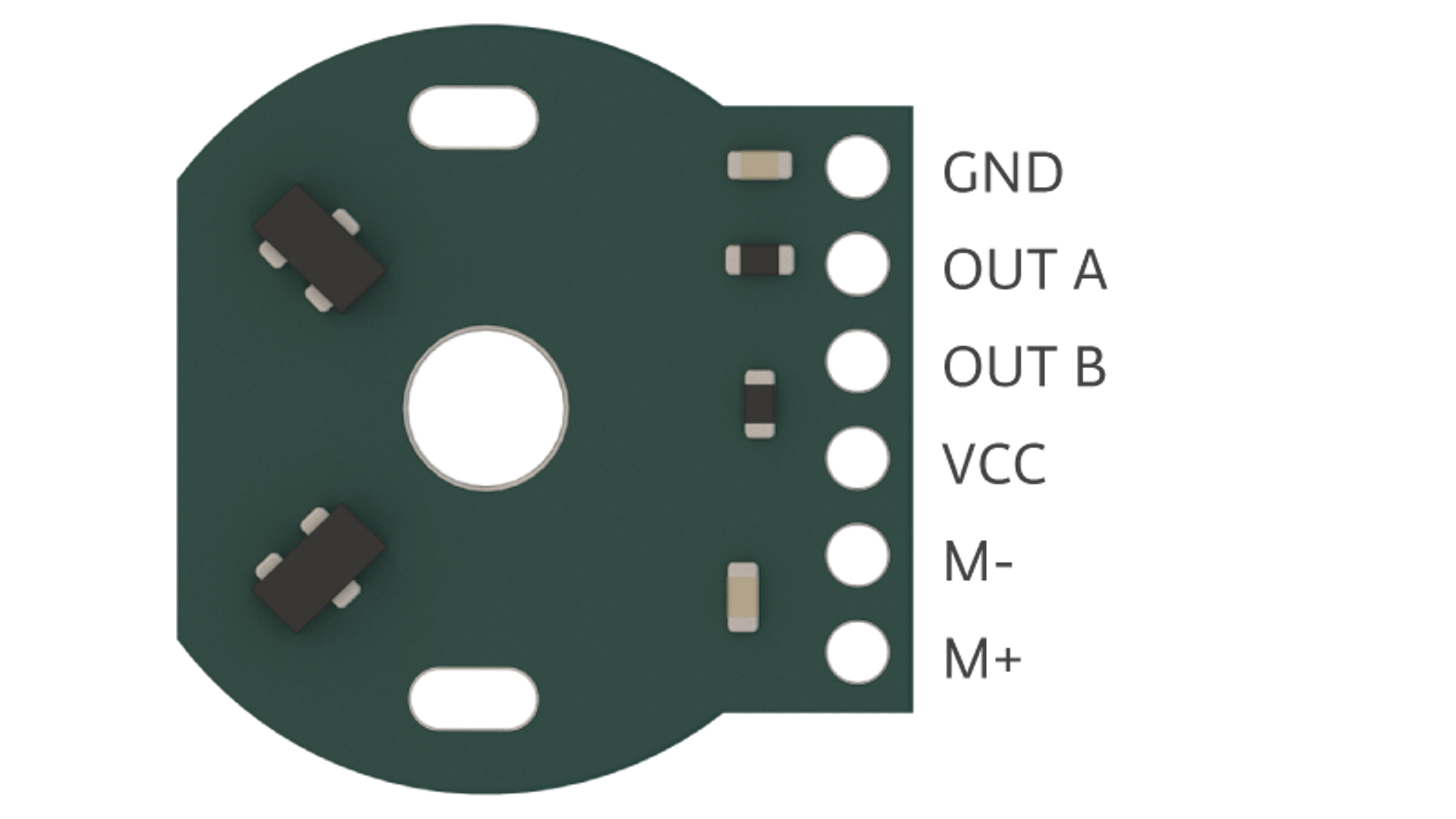
The provided motor has a pre-attached rotary encoder (you can read more about rotary encoders in Chapter 3) integrated circuit that we will discuss later. The rotary encoder chip has a 6-wire header:
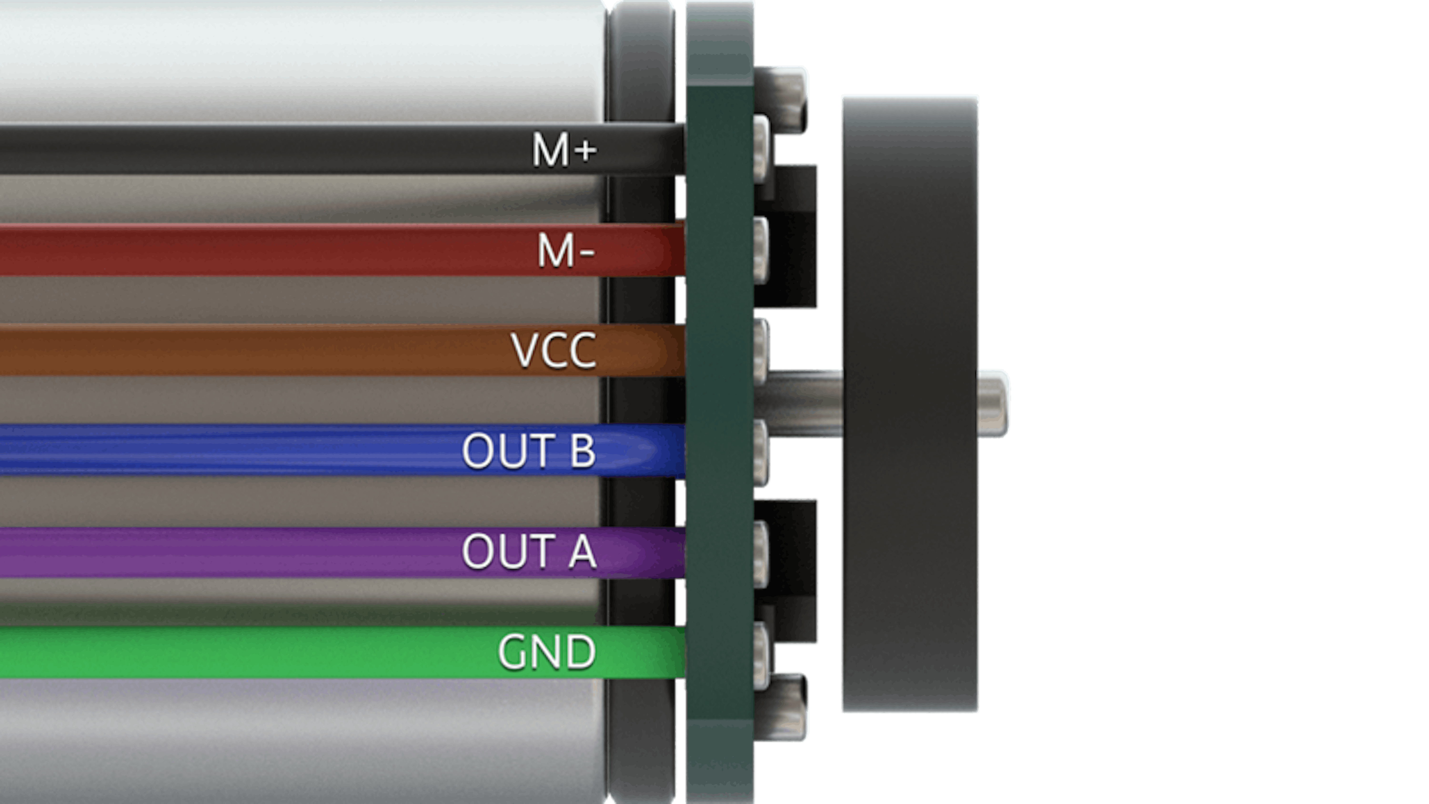
Note: In this case we are not following the naming convention for the cable colors. In the coming chapters, just follow the illustrations to know where to connect the cables.
The four wires called GND, OUT A, OUT B and VCC are related to the rotary encoder itself. The two wires labelled M+ and M- connect directly to the motor drive leads, which are hidden under the rotary encoder chip. Locate the ends of the two motor drive wires.
Torque is delivered to the motor by applying a voltage across these two wires. The magnitude of the voltage corresponds to the amount of torque applied, and the sign of the voltage is analogous to the direction of the applied torque.
On the Motor Carrier, locate the headers for DC motor M3. You should see the labels M3+ and M3- printed on the Motor Carrier board next to the corresponding screw terminals.
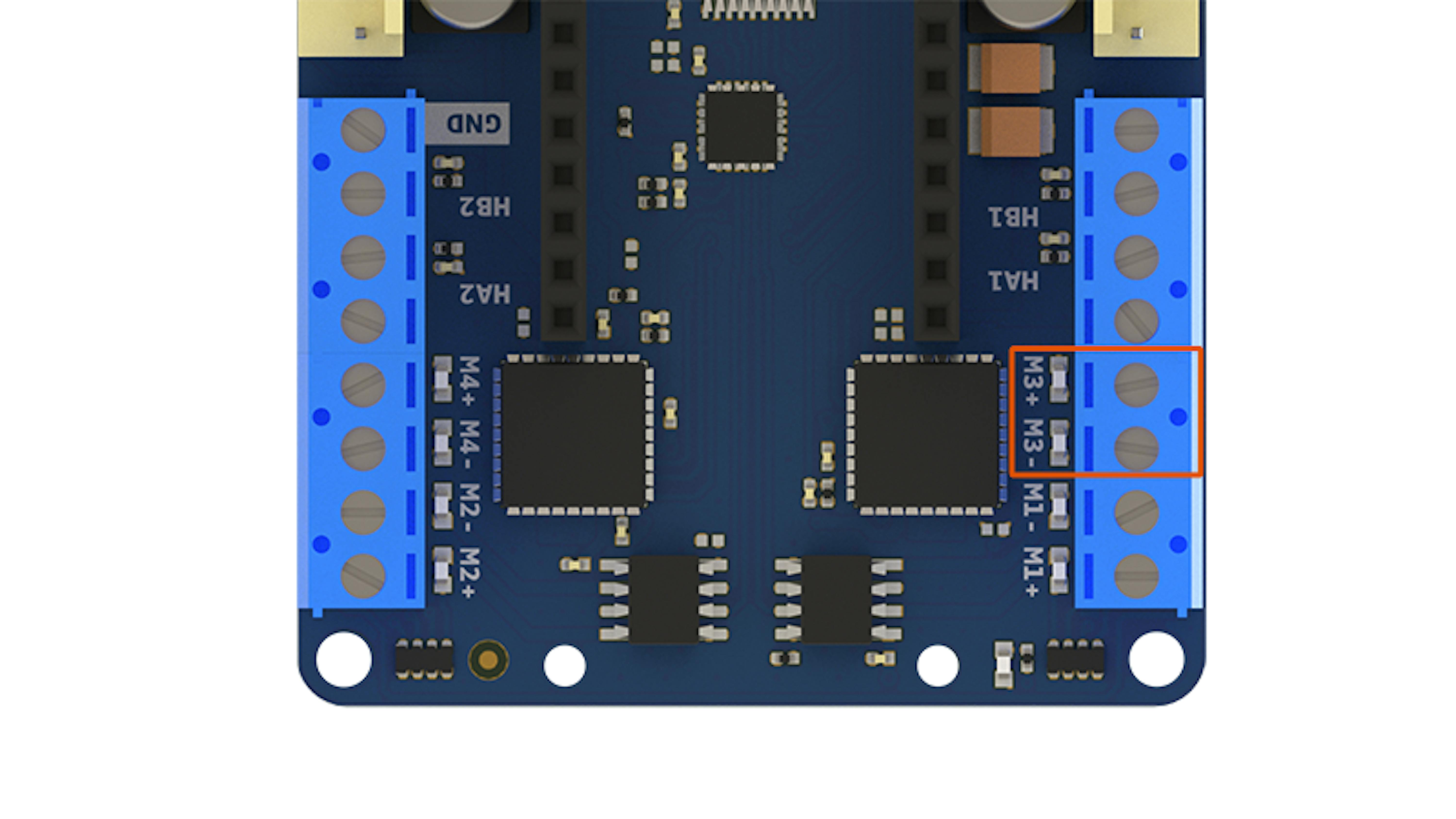
Using a small flathead screwdriver, insert the right-most wire marked M+ from the DC gearhead motor into screw terminal M3- and tighten the screw until the wire is securely fastened (gently pull on the wire to make sure it is secure). Similarly, fasten the second right-most wire marked M- from the DC gearhead motor into screw terminal M3+.
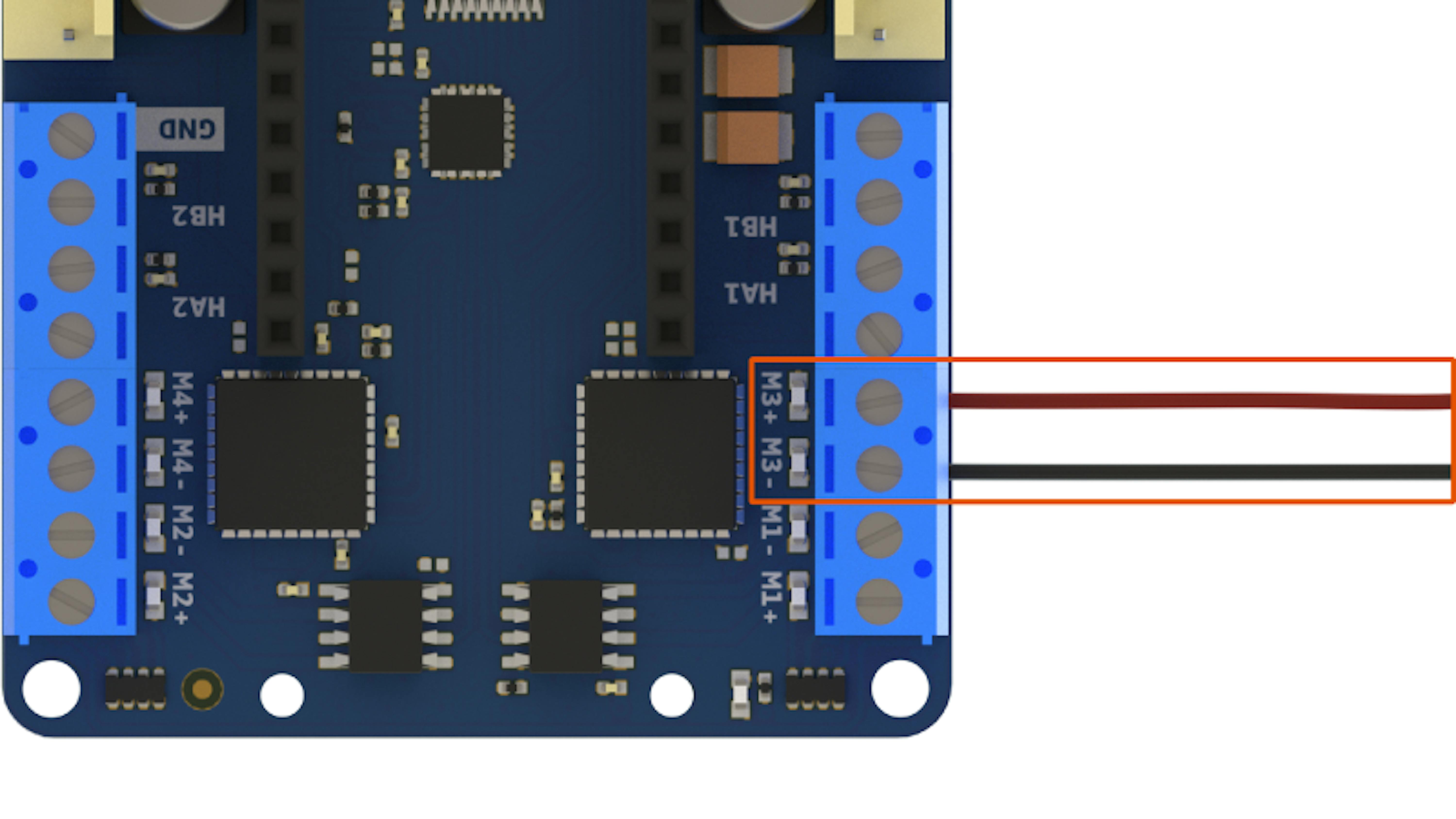
Note: the signs of the wire (M+) and the screw terminal (M3-) are intentionally different.
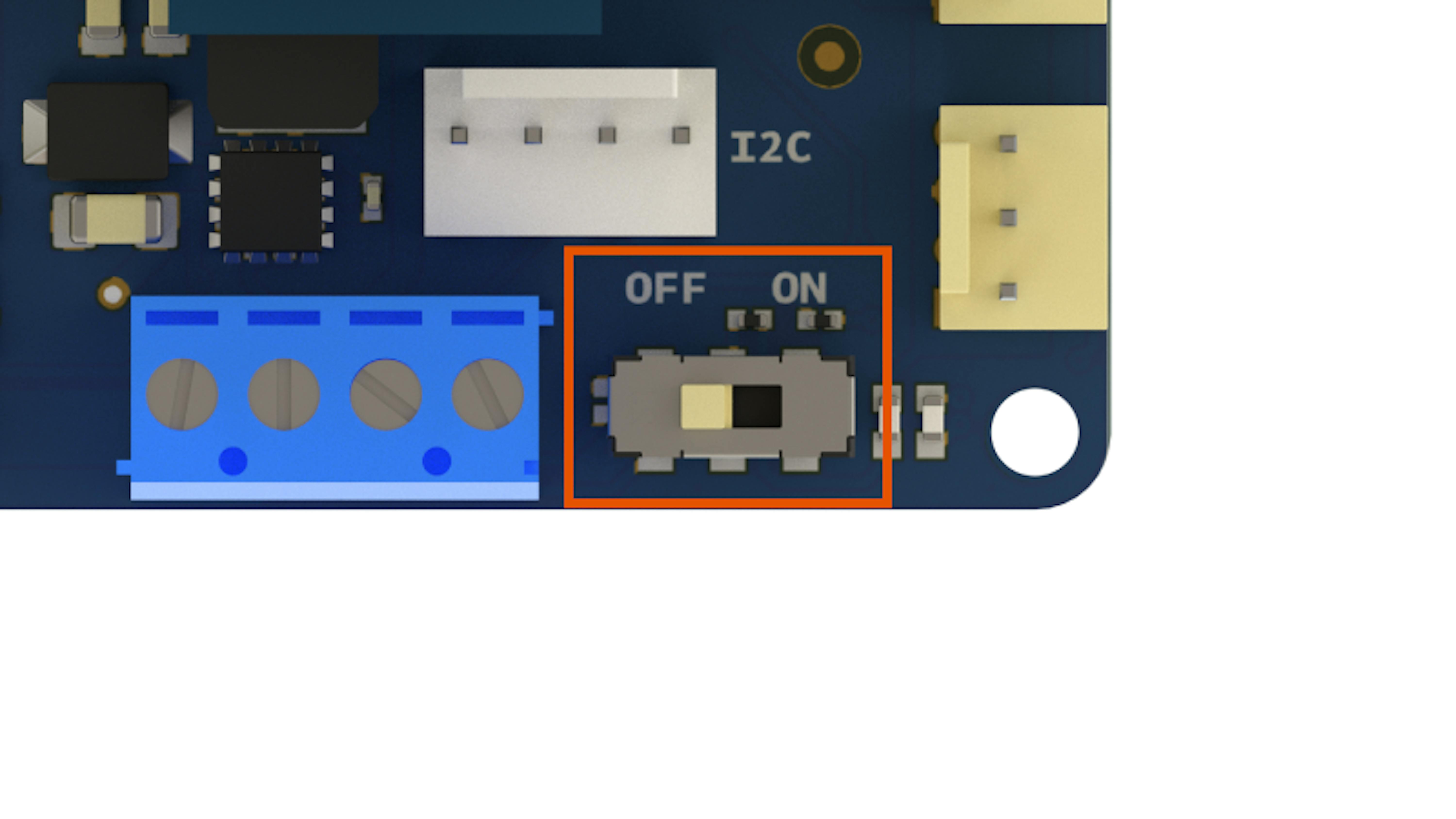
Next, locate the power switch on the Motor Carrier and ensure that it is set to OFF.
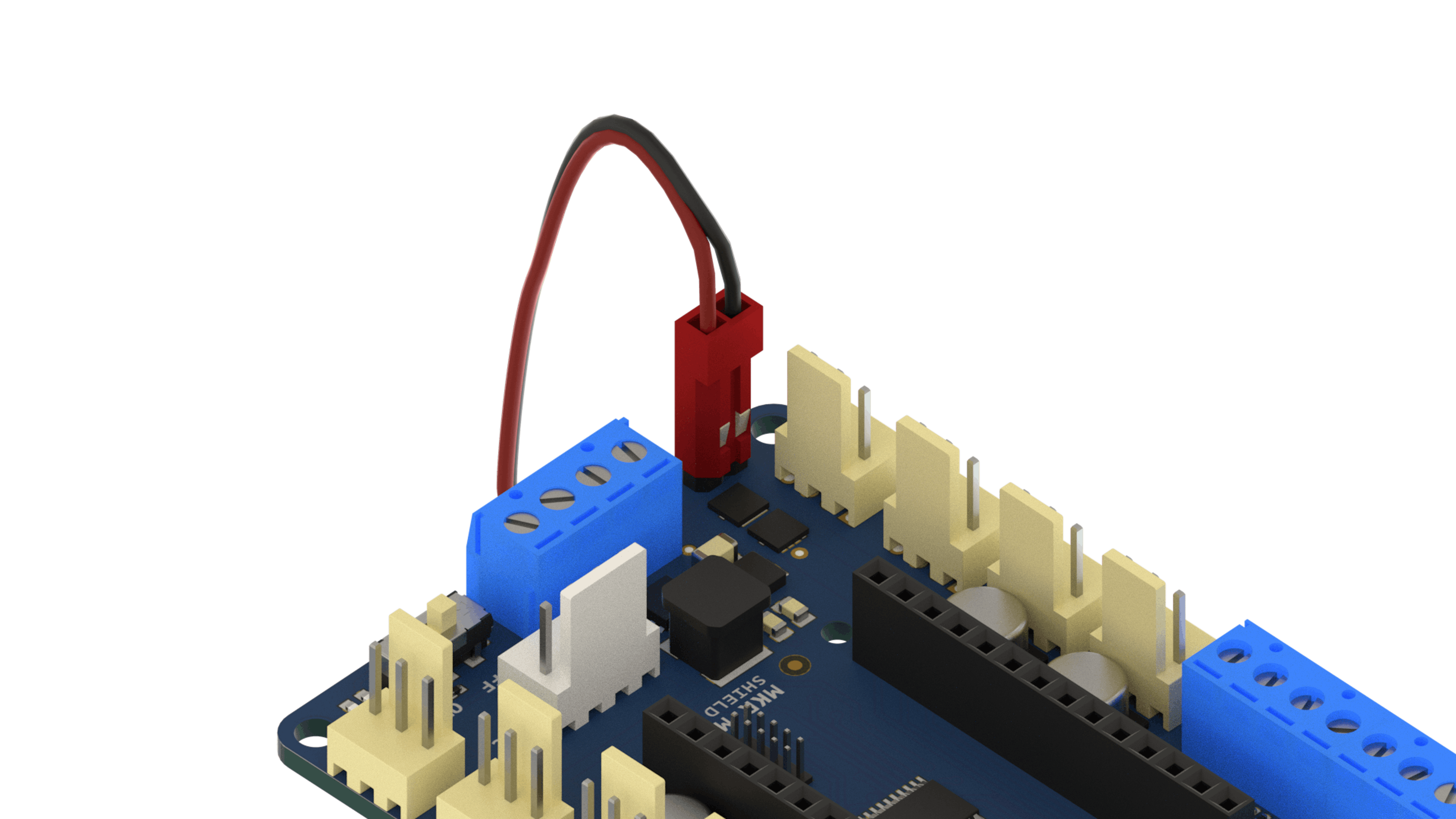
Now locate your LiPo (Lithium Polymer) battery and attach it to the battery header on the Motor Carrier as shown. Ensure that the black wire is aligned with GND and the red one is aligned with VIN to ensure the correct polarity:
Plug in the USB cable again, switch the Motor Carrier power switch to ON, and ensure that the nearby LED illuminates:

As you switched the MKR1000 board's power source from USB to LiPo battery, you must re-establish your MATLAB connection to Arduino. Run the following commands to do so:
>> clear a
>> a = arduino
Now let's create a second MATLAB object to provide access to the MKR Motor Carrier. Use the following command to create a Carrier object in the MATLAB Workspace that is associated with the Arduino object a :
>> carrier = addon(a, 'Arduino/MKRMotorCarrier')
Just as the MKR Motor Carrier provides a physical interface between the motor drive wiring and the MKR1000 board, the carrier object is an intermediary between the Arduino object and the DC and servo motors we may connect.
The Motor Carrier allows you to drive your motors with a relatively powerful battery. This can provide much larger currents than the Arduino board itself, which derives all its power from the USB connection to your computer. The USB port cannot provide enough current to drive motors at the necessary voltage, and it can be dangerous to attempt to do so.
Now let's create a third object to give you control of the motor connected to M3 in MATLAB. Use the following command to create a DC Motor object that is associated with the Carrier object, and examine the displayed object properties in the Command Window:
>> dcm = dcmotor(carrier,3)Now you can drive the motor. You can see that DC motor object has three properties MotorNumber, DutyCycle and IsRunning. You can change the DutyCycle property directly by assigning values between -1 and 1. You can control the IsRunning property using the methods start and stop. Try the following commands to control the motor speed:
>> start(dcm)


>> dcm.DutyCycle = 0.5;


>> dcm.DutyCycle = 0.3;


>> dcm.DutyCycle = -0.3;


>> dcm.DutyCycle = -0.1;


>> dcm.DutyCycle = -0.05;


>> dcm.DutyCycle = -0.01;


>> dcm.DutyCycle = -0.3;


>> stop(dcm)


>> start(dcm)


>> stop(dcm)


>> dcm.DutyCycle = -0.5;


>> start(dcm)


>> stop(dcm)
The voltage applied to the DC motor is controlled by a PWM signal (you can read more about PWM signals in Chapter 3). The magnitude of dcm.DutyCycle indicates the duty cycle of the PWM signal. When dcm.DutyCycle is positive, the PWM signal multiplies the battery's potential difference to produce some positive fraction of the battery's voltage rating. When dcm.DutyCycle is negative, the same multiplication occurs but the "reference" and "ground" voltages are reversed in the circuitry. As a result, a negative fraction of the battery's voltage rating is applied to the motor and negative torque is applied.
You may have observed that there is a dead band when dcm.DutyCycle is very close to 0. This is because the applied torque is not large enough to overcome the static friction in the various axles in the gearbox. This is something that should be considered when designing a motor control system.
ROTARY ENCODER: POSITION AND SPEED
Let's shift gears (metaphorically) and talk about sensors. In the Concepts chapter in Section 3.3, you can read how a rotary encoder uses two digital signals to determine changes in rotational motion and accumulate them over time. Let's see how it is implemented here.
There are two pieces of hardware involved in measuring the rotational angle of the motor. First, the rotary encoder hardware, attached to the motor shaft, consists of an integrated circuit, which remains stationary, and a magnetic disk, which rotates along with the motor shaft. As the magnetic poles rotate relative to the chip, they act on two electromagnetics within the chip such that they generate two digital signals A and B with the quadrature form discussed later in the Concepts chapter. These signals correspond to the wires labelled OUT A and OUT B on the rotary encoder chip, as shown in the image below. The wires GND and VCC are for ground and voltage input, respectively. They will be connected to a supply voltage source so that current can be provided to generate the A and B signals. As an exercise, identify these four wires on your MKR Motor Carrier.
Second, the MKR Motor Carrier contains a data buffer for each of the two encoder ports. Each time the A or B signal changes from the encoder chip, the value in the data buffer is incremented or decremented by one. The resulting integer value is the encoder count, which we can read any time we need it.
Switch the MKR Motor Carrier power to OFF and disconnect the USB cable. Attach the encoder wires to the corresponding screw termi
Connect the USB cable and power on the MKR Motor Carrier and then create a MATLAB object to access the rotary encoder count buffer at encoder port 1, using the following commands:
>> clear a
>> a = arduino
>> carrier = addon(a, 'Arduino/MKRMotorCarrier')
>> dcm = dcmotor(carrier,3)
>> enc = rotaryEncoder(carrier,1)
To read the encoder count buffer, use the following command, and note the result:
>> readCount(enc)The geometry of this encoder is such that there are three full cycles of quadrature when the motor shaft turns one full revolution. Recall that the quadrature signals undergo four total changes in a full cycle. This means that there are 12 quadrature signal changes per revolution for the motor shaft. Thus, we can measure the angular position of the motor shaft with a resolution of 30 degrees, if we know the encoder count. Manually rotate the magnetic disk one full clockwise revolution (when looking down on the magnetic disk), and read the encoder count again:
>> readCount(enc)What is the change in encoder count? If your encoder was wired as instructed, you should have seen the count increase between readings. If the outA and outB pins on the encoder were wired the opposite way, the count would have decreased between readings. From a purely electrical point of view, there is no right or wrong way to wire the encoder; you just need to be aware of this fact and take it into account when you calibrate the sensor.
Just to confirm that everything works as expected, rotate the magnetic disk one full counterclockwise revolution. What is the change in encoder count? Once more, if the encoder was wired as instructed, the values would decrease between readings; if the wiring was the opposite, the values would increase. If your application uses only changes in rotation over a span of time, then it does not matter what the initial value is in the encoder count buffer. However, if your application requires knowledge of absolute rotation from the start of execution, it is useful to reset the count to zero. Enter the following commands to read the current encoder count, reset the buffer, and reread the count:
>> readCount(enc)
>> resetCount(enc)
>> readCount(enc)
The chosen encoder hardware provides a resolution of 12 counts per motor shaft revolution (see technical specifications at this link). Thus, you can convert the motor shaft's encoder count to the physical angle of the motor shaft in degrees as follows:
>> shaftAngle = readCount(enc)*360/12This DC motor has a gear ratio of 100.37:1 (see technical specifications at this link) between the motor shaft and the output shaft that attaches to the device you're driving, such as a wheel. Use the following commands to get the angle of the output shaft in degrees, and then normalize it to the range of 0 to 360 degrees:
>> axleAngle = readCount(enc)360/12/100.37
>> axleAngleNorm = mod(axleAngle,360
Now let's displace the output shaft angle using the DC motor rather than manual rotation:
>> dcm.DutyCycle = 0.5;
>> start(dcm)
>> readCount(enc)
>> readCount(enc)
>> readCount(enc)
>> stop(dcm)
Now you're able to determine the angle of the motor shaft and output shaft, and thus changes in angle over some interval of time. To get the angular speed, you need to also measure the duration of that interval. In MATLAB, you can measure elapsed time using the tic and toc functions. The first command, tic, will start a timer when issued; the second one, toc, will read the elapsed time since the last time tic was invoked. Try entering the commands below to understand how tic and toc work:
>> tic
>> toc
>> toc
>> dt = toc
>> tic
>> toc
>> toc
Now let's try the following: while we're measuring the change in encoder count, let the motor run. It is important that we measure the starting angle and start the timer simultaneously. To do this, we'll start the motor, and then do both actions in a single MATLAB command:
dcm.DutyCycle = 0.5;
start(dcm)
startCount = readCount(enc);tic
Next, read the encoder count again while simultaneously measuring the elapsed time, and then stop the motor.
stopCount = readCount(enc); dt = toc
stop(dcm)
Now let's determine the speed for the output shaft, first in counts per second, and then in degrees per second. Use the following commands:
>> speed = (stopCount - startCount)/dt
>> convSpeed = (stopCount - startCount)*360/dt/12/100.37
CHARACTERIZING A DC GEAR MOTOR IN MATLAB
In this section, you will write a MATLAB program that automatically measures the motor speed while issuing many different PWM commands to characterize the response of the 100:1 DC gearhead motor. Later, you will use these observations to determine the required PWM command to rotate the motor at a desired rotational speed. Using the Live Editor, you will compose a MATLAB live script that performs the following tasks:
In this section, you will learn:
- How to automate processes in MATLAB using a script.
- How to use code sections to partition scripts into smaller parts.
- How to use for-loops to repeat blocks of code.
- How to use text labels and comments to organize and document MATLAB scripts.
- How to create and call a MATLAB function.
WRITING MATLAB SCRIPTS
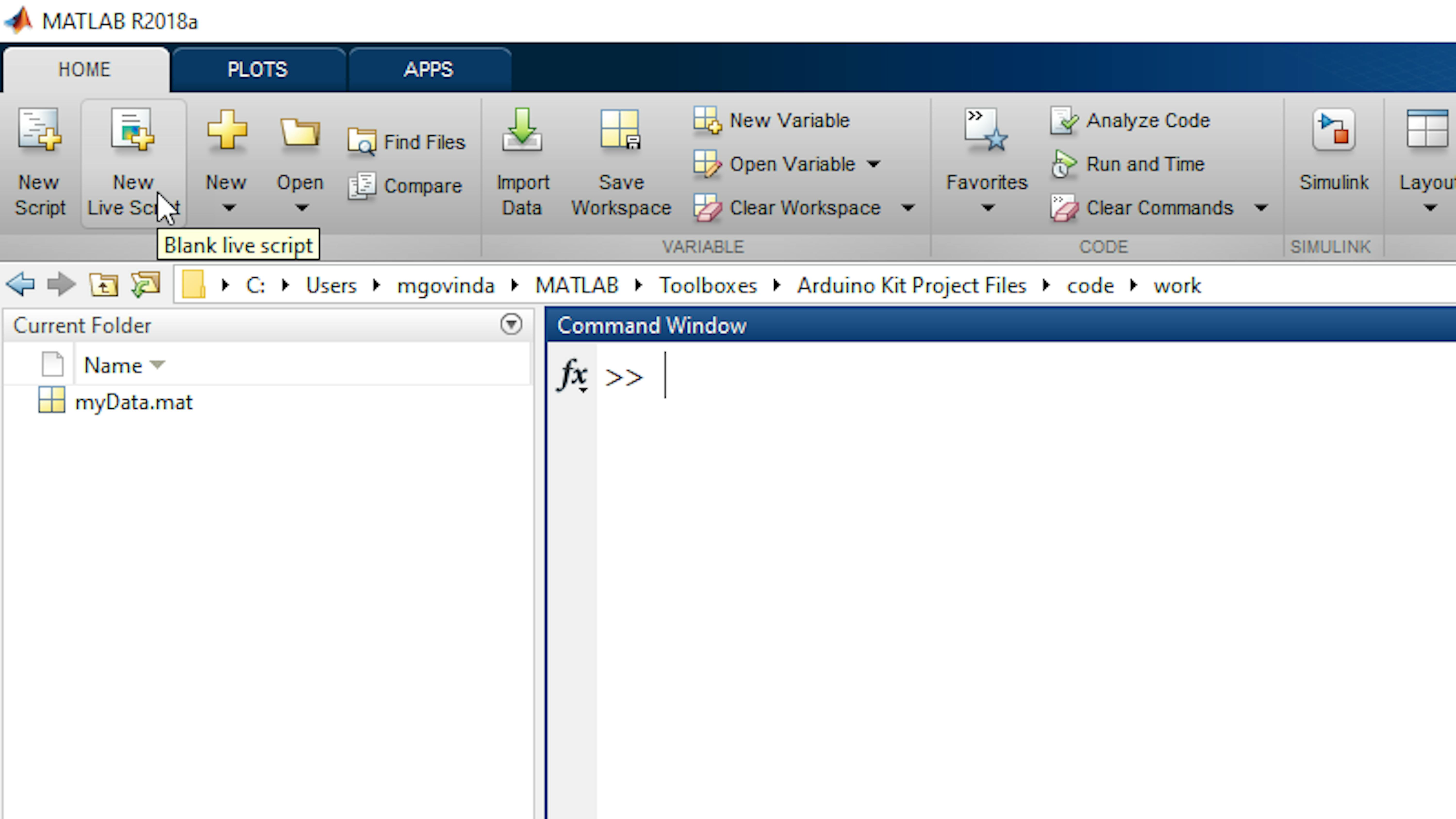
Up to this point, you have been typing commands directly on MATLAB's command line. If you perform certain operations many times, it might be useful to group those lines of code into scripts that you can easily call when needed. These are called live scripts in MATLAB's jargon. Begin by opening the Live Editor window. In the MATLAB Toolstrip , click New Live Script.
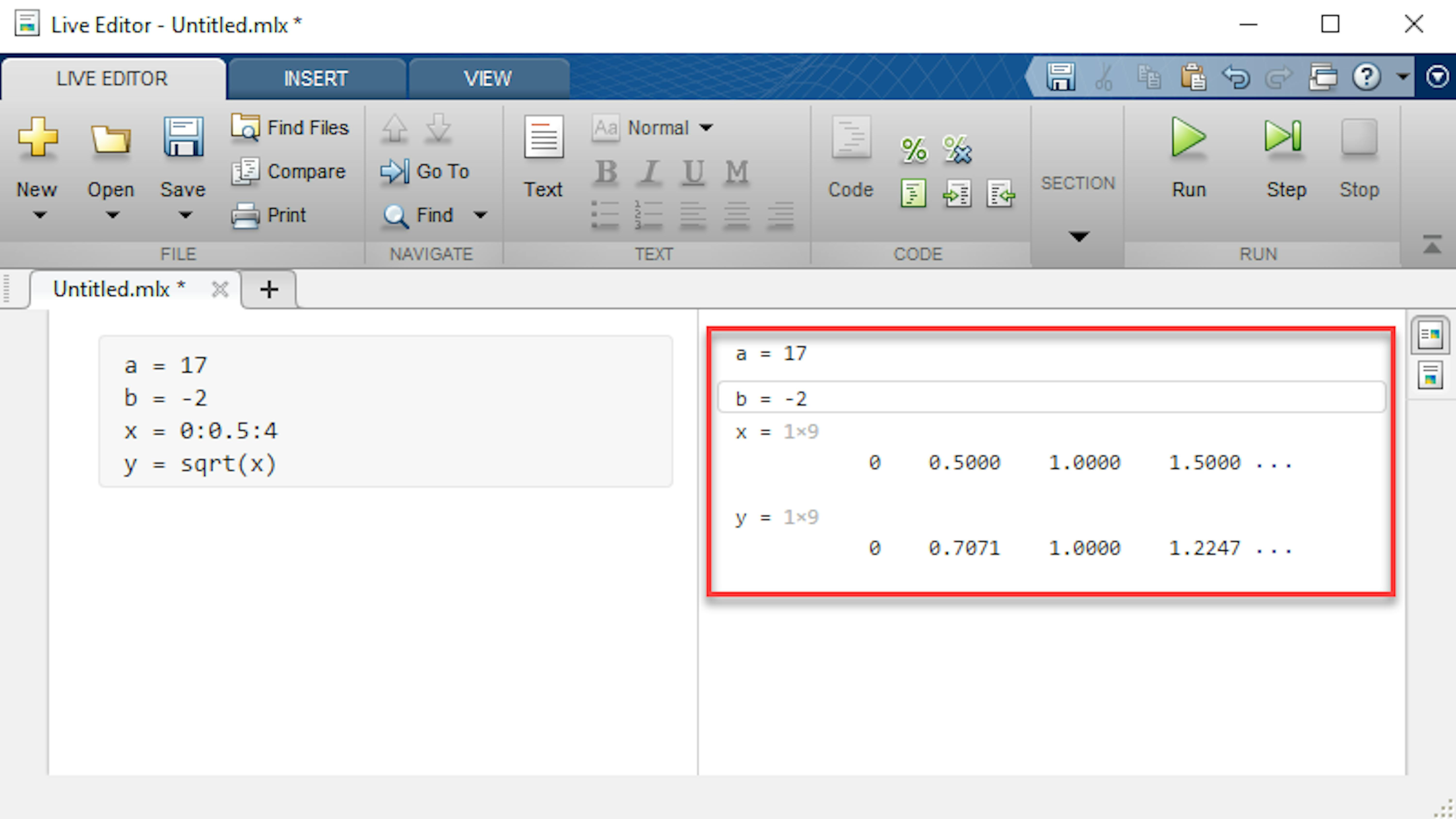
In the Live Editor window, you can type the same MATLAB commands as you would in the Command Window, and then execute them in batches. Start your live script by typing a few simple lines of code:
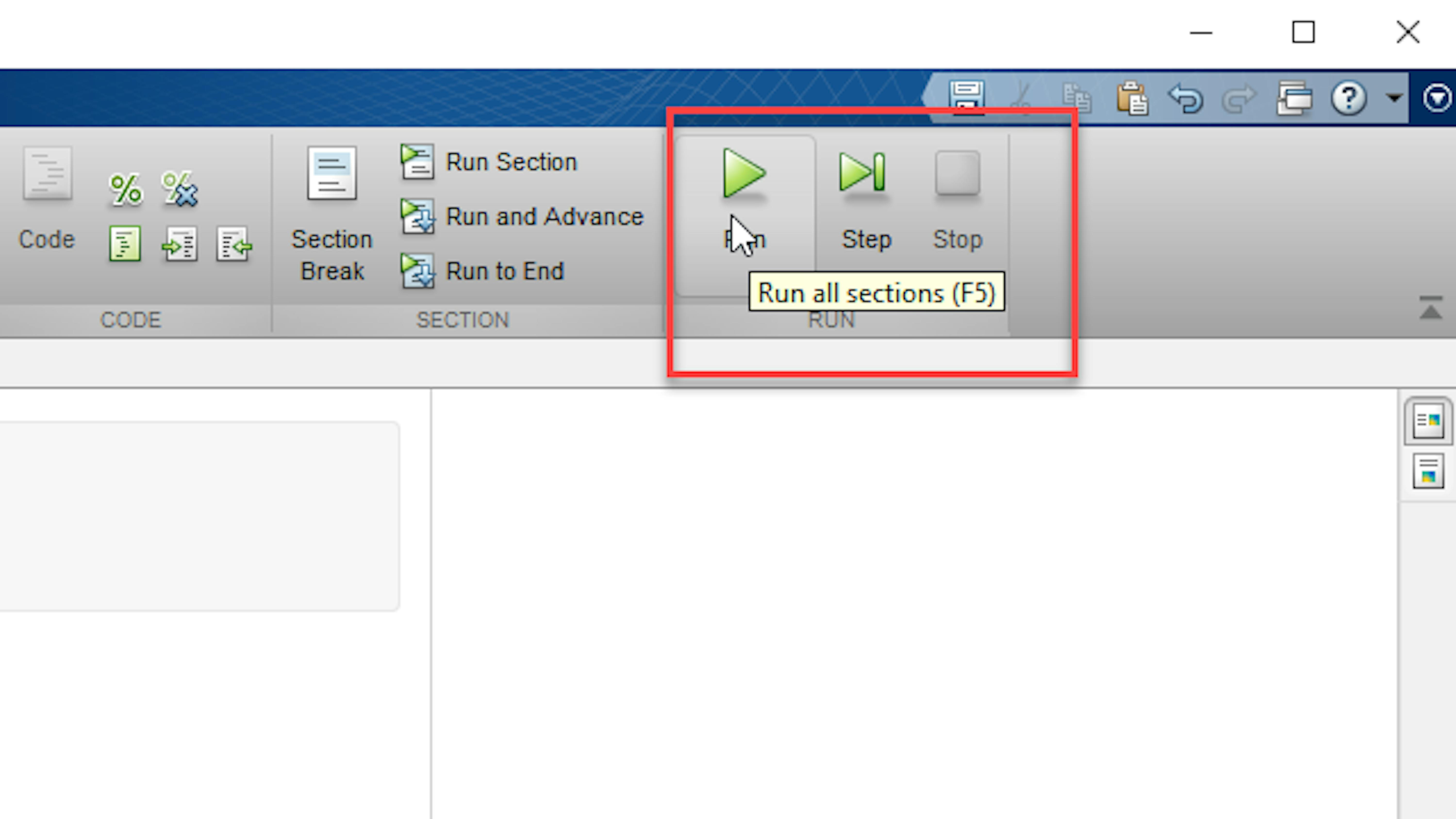
Execute your live script by clicking Run:
a = 17
b = -2
x = 0:0.5:4
y = sqrt(x)
Execute your live script by clicking Run:

Your commands execute sequentially, and assignment expressions modify variables in the MATLAB Workspace. Examine the Workspace and locate the new variables. As you can see, the results of expressions with unsuppressed output are displayed in the right column:
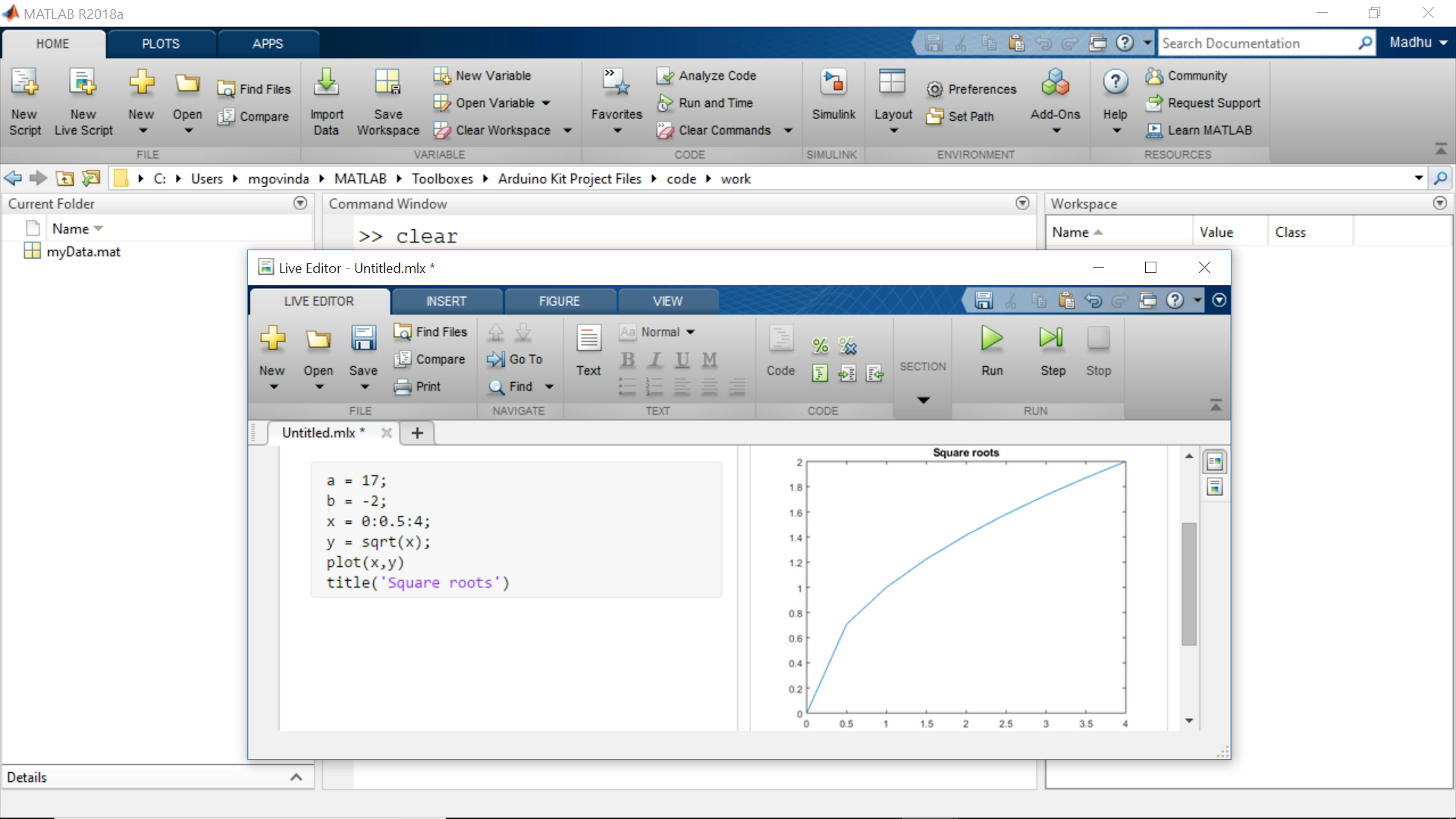
Now suppress the output (which consists of adding a semi-colon at the end of the command), and plot y against x by adding the code in bold:
a = 17;

b = -2;

x = 0:0.5:4;

y = sqrt(x);

plot(x,y)

title('Square roots')
Run the script and examine the embedded figure in the output column. Then clear your Workspace in the Command Window:
**>> clear**Now run your live script again:
Examine the Workspace . You can see which information is being sent back to the command line and which isn't, depending on whether the variables are suppressed or not. Now that you have learned how to use live scripts to execute series of commands multiple times, we can use that knowledge to work with DC motors and characterize their behavior in terms of the PWM signal applied to them.
SETTING UP ANALYSIS DATA
Let's begin writing our motor characterization program. Delete the existing code in your live script, and type the following lines to define your test PWM command values:
maxPWM = 1.00;
incrPWM = 0.05;
PWMcmdRaw = (-maxPWM:incrPWM:maxPWM)';
Run your live script and examine your Workspace. You have created a vector containing a series of numbers ranging from -1 to 1 with 0.05 increments. That will be used to generate the PWM signal we will apply to the DC motor to characterize its behavior.
CREATING ARDUINO AND EXTERNAL DEVICE OBJECTS
Now let's add some code to create and/or initialize the four device objects that we will need for this experiment: Arduino ( a ), the DC motor (dcm), the Carrier (carrier), and the encoder (enc). Add the following bold lines of code to your live script:
maxPWM = 1.00;
incrPWM = 0.05;
PWMcmdRaw = (-maxPWM:incrPWM:maxPWM)';
clear a dcm carrier enc
a = arduino;
carrier = addon(a,'Arduino/MKRMotorCarrier');
dcm = dcmotor(carrier,3);
enc = rotaryEncoder(carrier,1);
resetCount(enc);
Rerun your live script to ensure correct behavior; you can check the results by looking at the Workspace. If everything went as expected, your live script now includes all the objects needed to perform the test.
USING SECTIONS, TEXT, AND COMMENTS
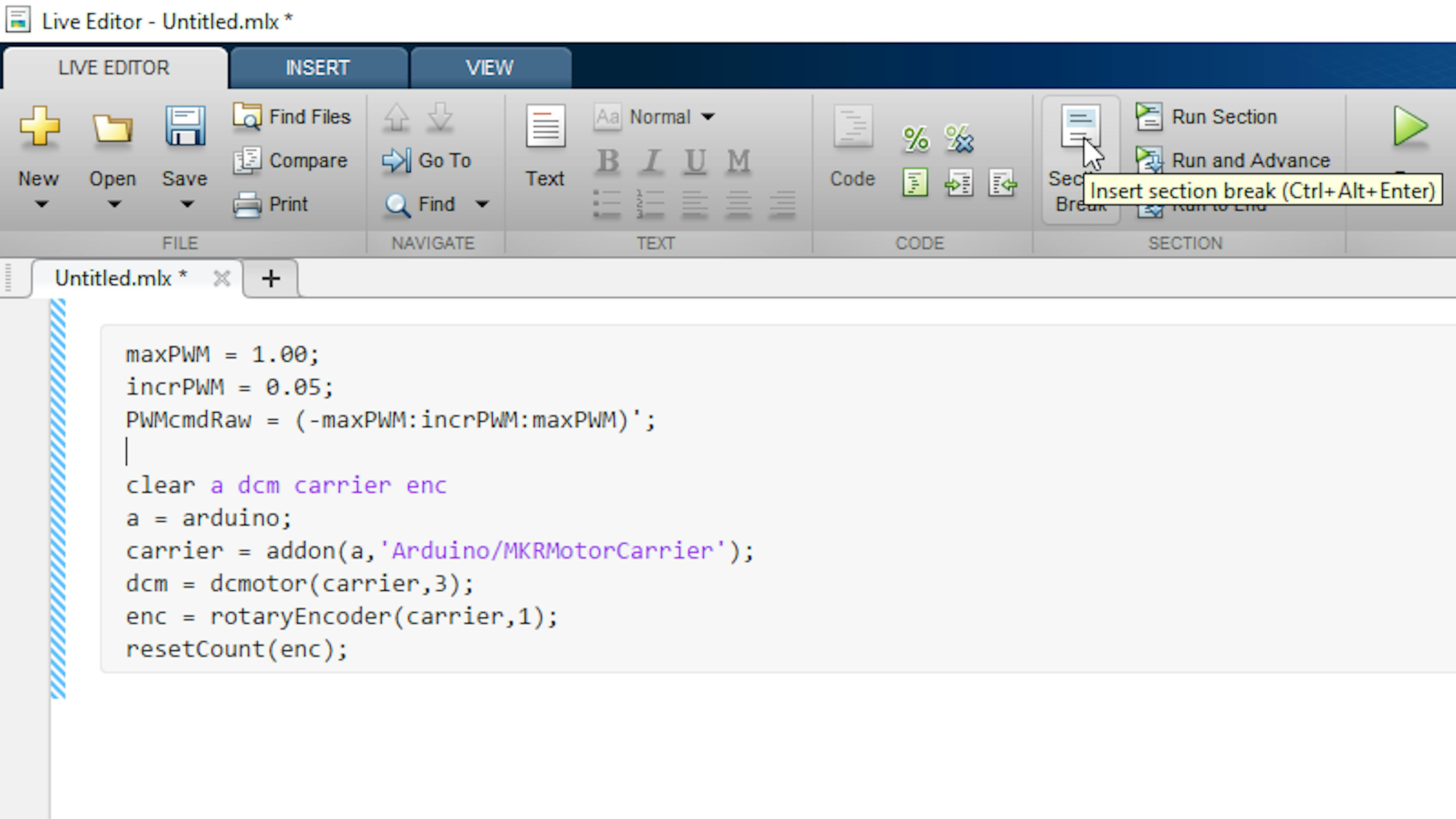
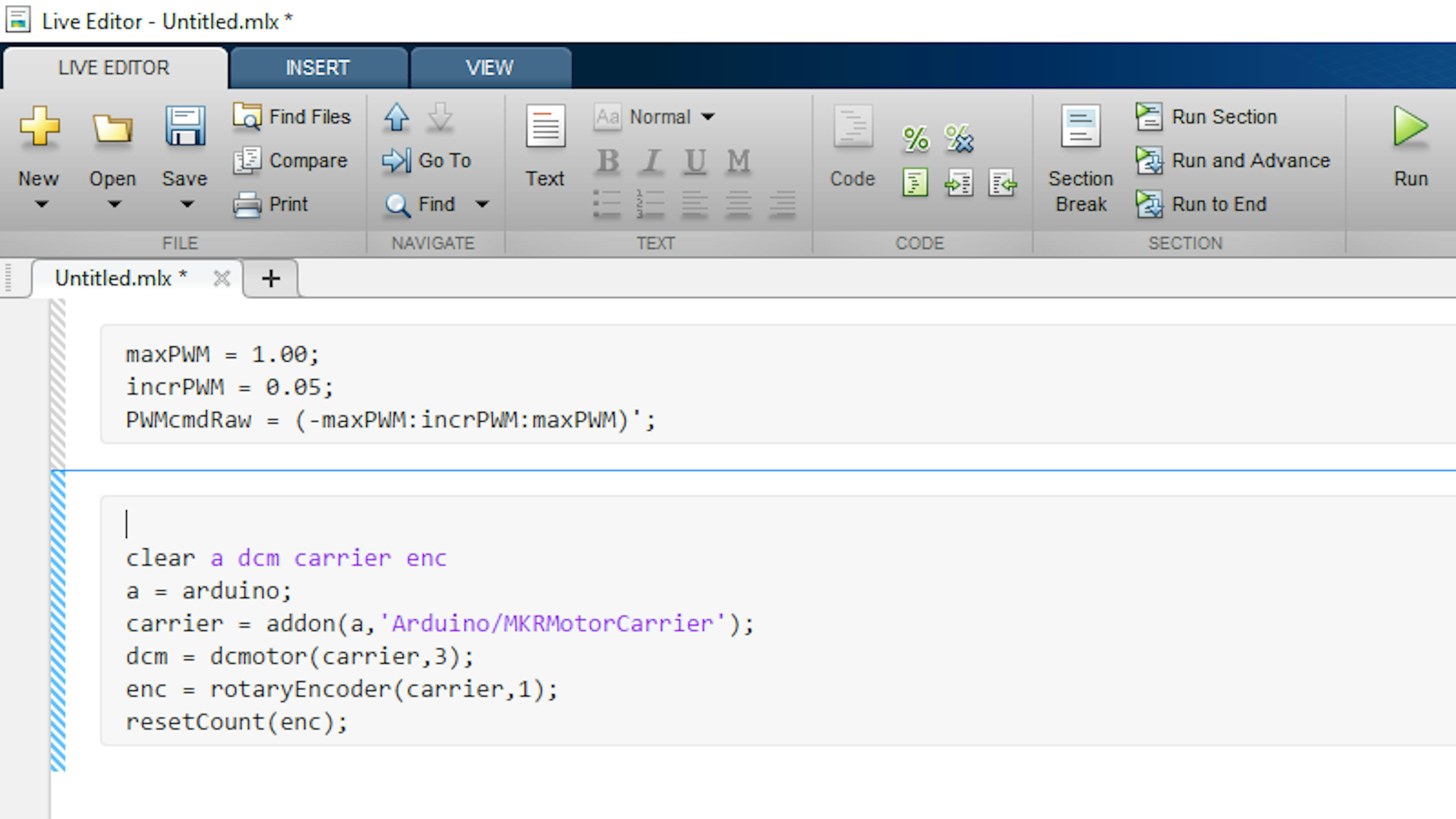
Before we proceed with the testing, let's make the script easier to understand for somebody less familiar with the program. First, you can break down the program into sections, to divide it into logical steps. To partition your code, place the text cursor immediately before the clear command, and click Section Break.
Next, let's add some labels to the sections of the live script to explain what each one does. Place your text cursor at the beginning of the document and click Text:
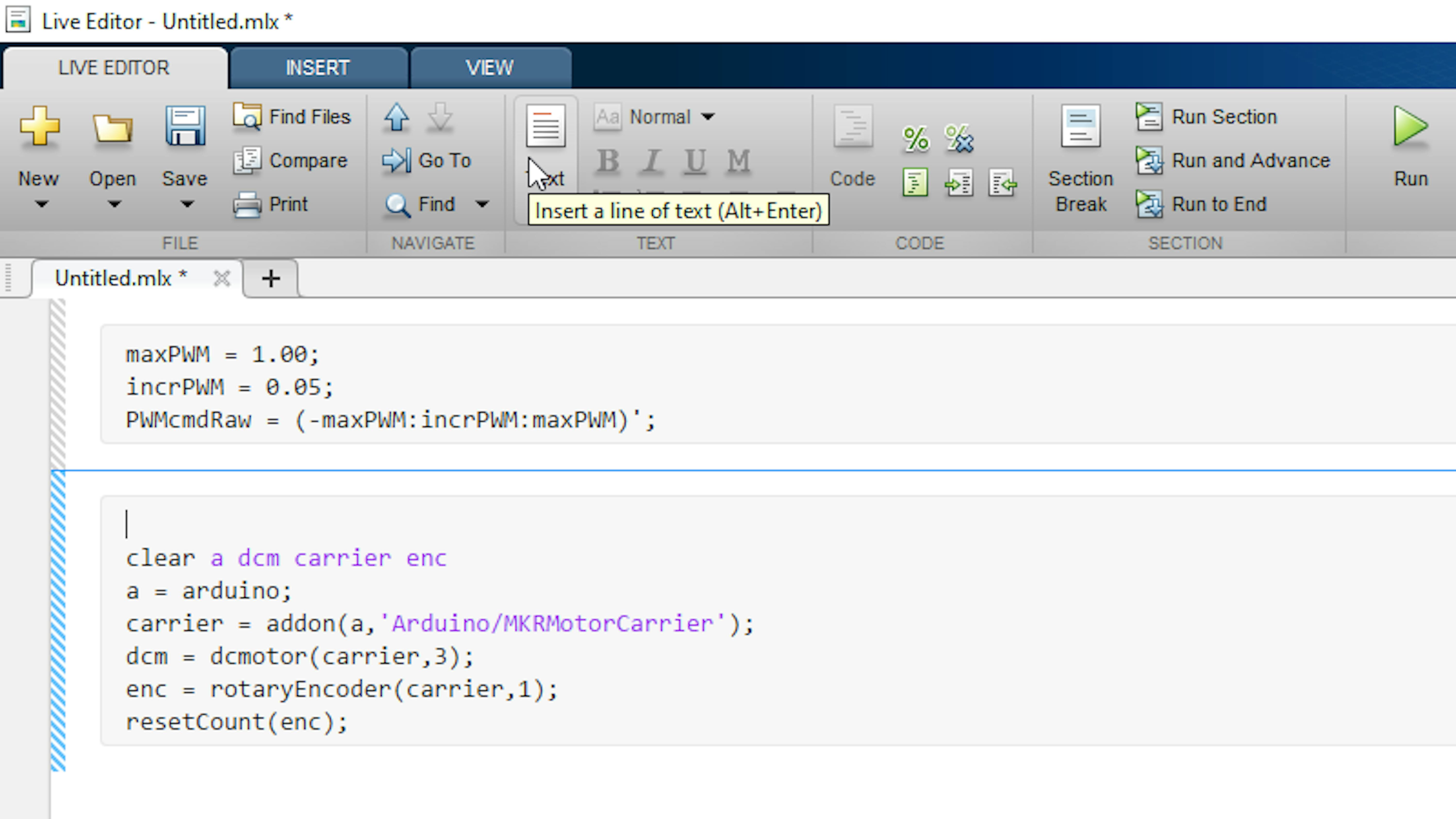
Now you can add a title and explanation for each section. Using plain text in the Live Editor, add the following labels. Use the formatting buttons in the Text panel of the toolstrip:
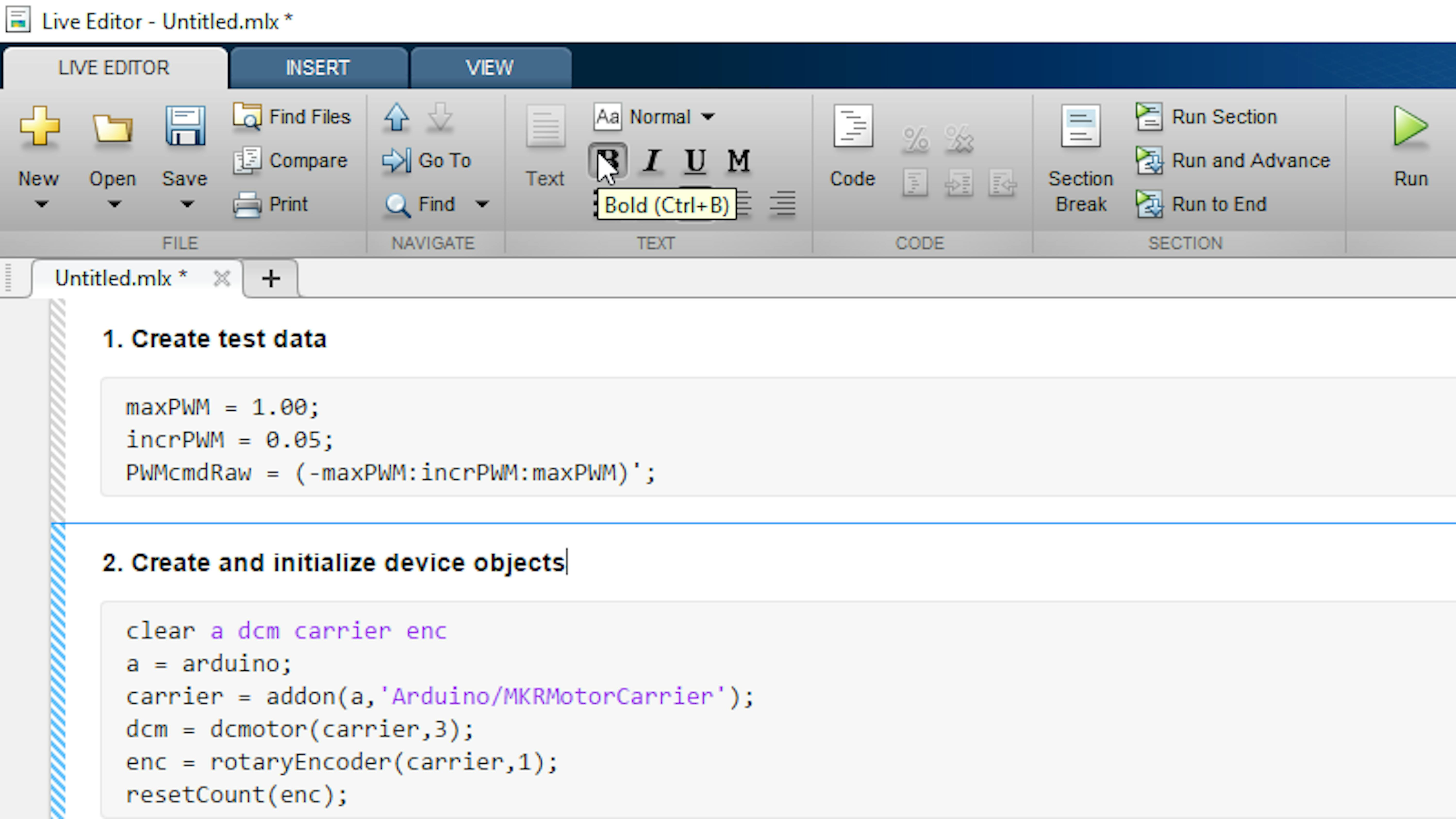
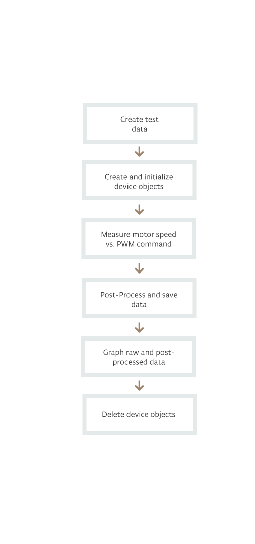
- Create test data
clear a dcm carrier enc% delete existing device objects

maxPWM = 1.00;
incrPWM = 0.05;
PWMcmdRaw = (-maxPWM:incrPWM:maxPWM)';- Create and initialize device objects
clear a dcm carrier enc

a = arduino;
carrier = addon(a,'Arduino/MKRMotorCarrier');
dcm = dcmotor(carrier,3);
enc = rotaryEncoder(carrier,1);
resetCount(enc);
Any portions of your live script that are written in plain text have no impact on how the script executes.
When you partition a live script into sections, you can execute each section one at a time. This can be useful if you want to just test one section without running the whole live script. You may also want to step through your code section by section, so that you can view and analyze intermediate results. Place your text cursor in the first section and click Run and Advance.
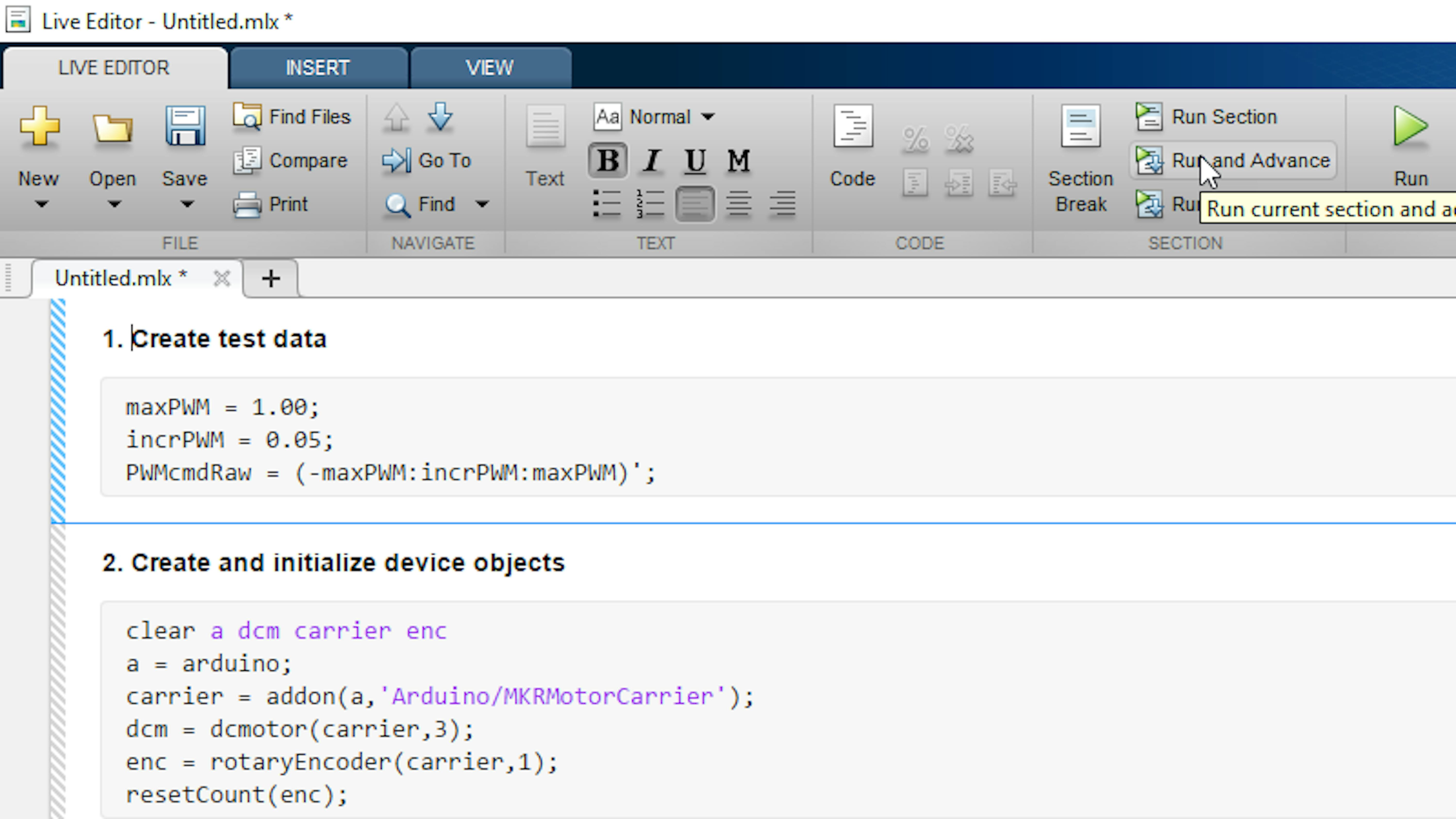
Click Run and Advance once more (or click Run Section or Run to End) to complete execution of the live script. Now clear your Workspace, and run your live script section by section, examining the Workspace after each section executes. You can also add comments to individual lines of code, if you want to add further explanation at a lower level. You can begin a comment directly in the MATLAB code by using the percent (%) character. Anything that follows % will not be executed in the live script. Add the following comments to existing lines of code:
- Create test data
maxPWM = 1.00;% maximum duty cycle
incrPWM = 0.05;% PWM increment
PWMcmdRaw = (-maxPWM:incrPWM:maxPWM)';% column vector of duty cycles from -1 to 1- Create and initialize device objects
clear a dcm carrier enc% delete existing device objects

a = arduino;
carrier = addon(a,'Arduino/MKRMotorCarrier');
dcm = dcmotor(carrier,3);
enc = rotaryEncoder(carrier,1);
resetCount(enc);
AUTOMATING MOTOR SPEED MEASUREMENT
After this short break where you learned how to better comment your code to make it easier to remember what each part of the code is doing, it is time to test the motor's behavior. MATLAB helps in automating tests. Previously, you have prepared the code by creating the objects that connect to Arduino, the Motor Carrier , and the encoder.
Now you will add a new section of code that starts the motor with a PWM value, reads the encoder count at two different times, derives the speed, and stops the motor. Add the following section to your live script to measure the speed for the first PWM value:
- Measure raw motor speed for each PWM command
dcm.DutyCycle = 0;
start(dcm) % turn on motor
resetCount(enc);
startCount = readCount(enc);
tic;
dcm.DutyCycle = PWMcmdRaw(1);
pause(1) % wait for steady state
stop(dcm);% turn off motor
dt = toc;
endCount = readCount(enc);
speedRaw(1) = (endCount - startCount) / dt; % calculate speed (cts/s)
dcm.DutyCycle = 0;
Try running this section with different index values of PWMcmdRaw and speedRaw. In the example code, the index is 1; we take the first index of PWMcmdRaw, send it to the motor, make two readings, and store the speed resulting from the calculation in the first element of speedRaw. Examine the results in the MATLAB Workspace.
ITERATING OVER MULTIPLE MEASUREMENTS
You now have a live script that you can use to get speed measurements for any PWM command value. Let's generalize this section of the script so that it measures the speed for all the values in the vector PWMcmdRaw. You can repeat parts of your code using a for-loop. A for-loop is a block of code that executes a known number of times, called iterations. To create a for-loop, you need a header (which defines the number of iterations), and the end keyword (which defines the end of the repeating code). A for-loop checks the value of an index variable to decide whether the condition to leave the loop has been met. The index indicates the current iteration. Here is a simple example of a for-loop:
**for** idx = 1:10
> y(idx) = (2 + idx) / idx;
**end**
This for-loop executes for 10 iterations, and the index variable idx takes a new scalar value from 1 to 10 during each iteration.
In our case, you want to iterate through all elements of PWMcmdRaw, and take a new speed measurement during each iteration. The result should be a vector that is the same size as PWMcmdRaw. Add a for-loop header and an end keyword to your code, as shown below. Remember to update the indices in PWMcmdRaw and speedRaw to the index variable, ii.
- Measure raw motor speed for each PWM command
dcm.DutyCycle = 0;
start(dcm)% turn on motor
**for** ii = **1:length(PWMcmdRaw)**
> resetCount(enc);
> startCount = readCount(enc);
> tic;
> dcm.DutyCycle = PWMcmdRaw(ii);
> **start(dcm)**% turn on motor
> pause(1)% wait for steady state
> stop(dcm); % turn off motor
> dt = toc;
> endCount = readCount(enc);
> speedRaw(ii) = (endCount - startCount) / dt;% calculate speed (cts/s)
> **pause(1)**;
**end**
**stop(dcm)** % turn off motor
dcm.DutyCycle = 0;
Run the section and ensure that all possible PWM values in PWMcmdRaw are tested. At this point, the Live Editor window should be showing a warning on the assignment to speedRaw(ii). Hover over the speedRaw variable in the Live Editor window to see details about the warning:
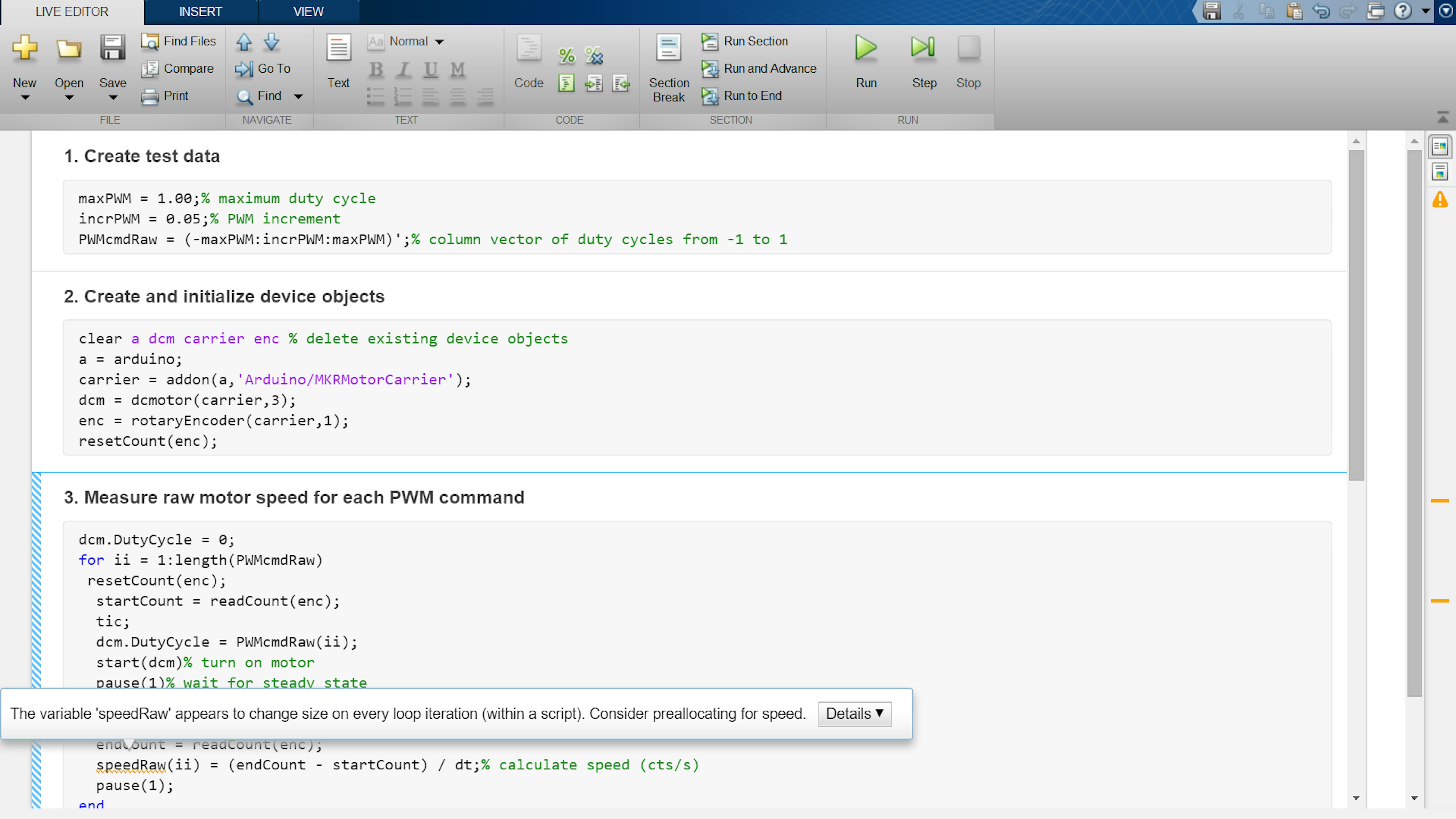
The warning appears because the script is assigning values to increasing indices of speedRaw, and as a result speedRaw needs to increase its size on every iteration to accommodate the new element. In some cases, this can lead to performance issues because the variable's memory may need to be reallocated many times. You can solve this problem if you know how large the array is going to get by defining the vector in advance.
Before assigning values to an array inside a for-loop, you should allocate memory for the array, so that it will not get resized inside the loop. The zeros function is often used for this purpose. Add the following bold line of code before the for-loop to allocate space for speedRaw before populating it with values:
- Measure raw motor speed for each PWM command
**speedRaw = zeros(size(PWMcmdRaw));** % Pre-allocate vector for speed measurements

dcm.DutyCycle = 0;

start(dcm)% turn on motor

**for** ii = 1:length(PWMcmdRaw)

>resetCount(enc);

>startCount = readCount(enc);

>tic;

>dcm.DutyCycle = PWMcmdRaw(**ii**);

>start(dcm)% turn on motor

>pause(1)% wait for steady state

>stop(dcm);% turn off motor

>dt = toc;

>endCount = readCount(enc);

>speedRaw(ii) = (endCount - startCount) / dt;% calculate speed (cts/s)

>pause(1);

**end**

stop(dcm)% turn off motor

dcm.DutyCycle = 0;
VISUALIZING MEASURED SPEED VS. PWM DUTY CYCLE
Now you have some real speed measurements in your Workspace. Let's visualize them against their corresponding PWM command values using the plot command we learned about earlier. Add the following section to your live script to plot and annotate the raw data:
- Graph raw data
plot(PWMcmdRaw,speedRaw)% raw speed measurements
title('100:1 Gearbox Motor Steady State Response')
xlabel('PWM Command')
ylabel('Measured Speed (counts/sec)')
Run the section and examine the figure in the output column of the Live Editor:
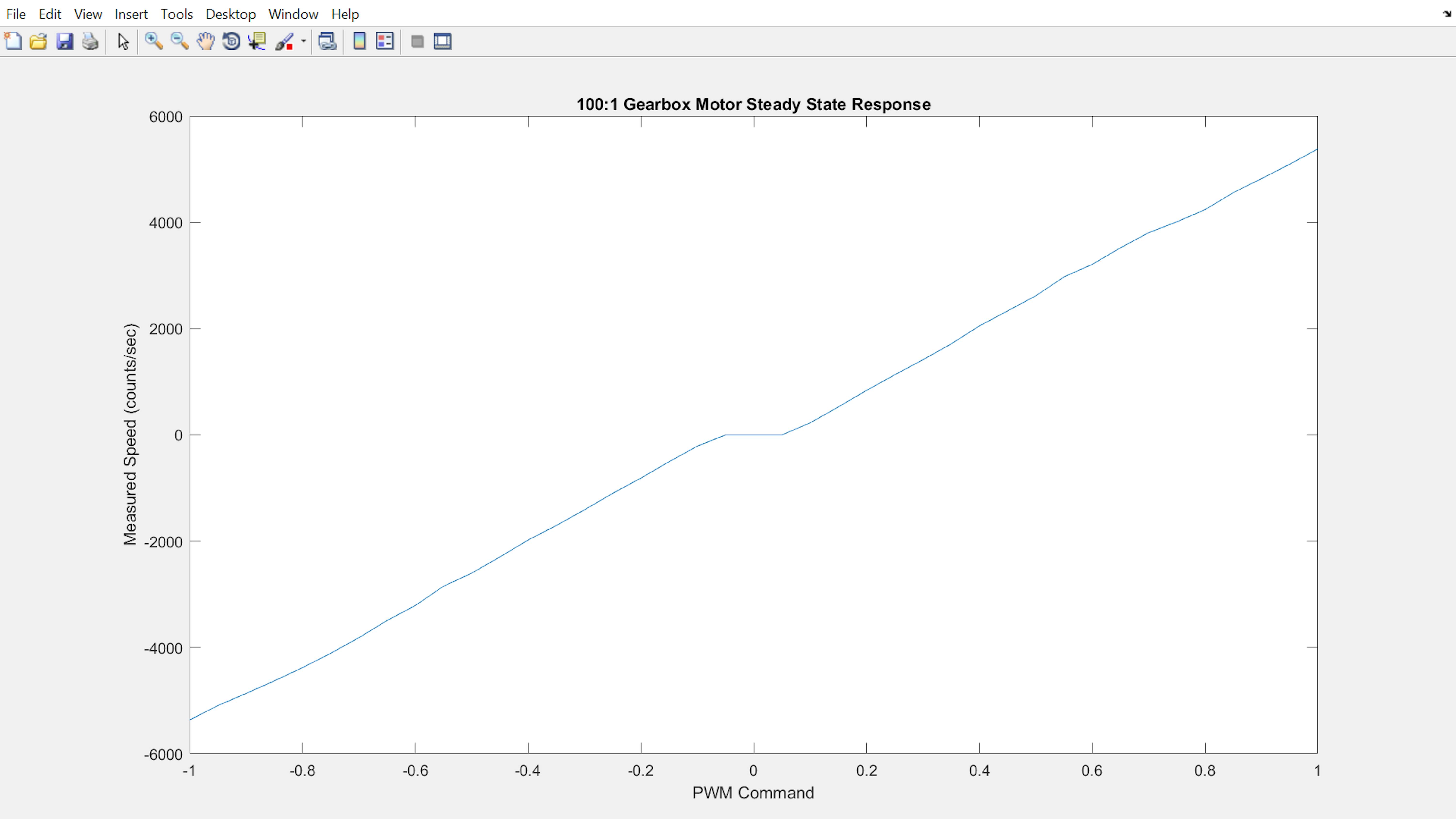
Notice some interesting features of the speed-PWM relationship that you can deduct from studying the graph. There is a "dead zone" around PWM=0, where there is zero rotational speed for non-zero PWM commands. Furthermore, there may be some non-monotonic portions of the curve, where the measured speed does not increase with increasing PWM command. This typically happens around PWM = +/-1, but could also result from experimental error.
POST-PROCESSING SPEED MEASUREMENTS
Collecting this data will be relevant later when you want to model how a more complex machine that uses several motors behaves. Later you will create a motor control system in Simulink, in which a user will request a motor speed in counts per second. The system will calculate the required PWM command to run the motor at that speed and send it to the Arduino board. To perform this operation correctly, the controller needs a one-to-one mapping between motor speeds and PWM commands. This means that there can only be one PWM command per speed, so you must remove repeated values and nonincreasing values from the data. First you must identify which values of speedRaw are not in increasing order. Examine speedRaw in the Command Window:
>> speedRawLocate the multiple zeros in the speed measurements and look for nonincreasing values.
It is not easy to see where the nonincreasing values are, so let's make a first-order difference. Enter the following command:
>> diff(speedRaw)This will answer with yet another vector showing the differences between pairs of values in the array. To remove non-increasing values in speedRaw, you need to know the indices where diff(speedRaw) is nonpositive. To do this, you can use relational operators to create a logical condition. Enter the following logical expressions, and interpret the result:
>> pi > 3

>> pi >= 3

>> pi == 3

>> pi < 3

>> x = 1:5

>> x == 3

>> x < 3

>> y = x < 3
For the first half of the previous commands (all the ones related to pi), the operations will produce a different result based on the level of truth of the statement.
For the second set of operations (the ones related to the variables x and y ), the results are different, since x is an array containing the numbers 1 to 5. Examine x and y in your Workspace. The numeric vector x is the same size as the logical index vector y. You can use a logical index expression or variable to index into a variable of the same size. Try the following commands:
>> x(y)

>> x(~y)

>> z = rand(1,5)

>> z(y)
Now let's get the logical indices and values of speedRaw where it is strictly increasing. Enter the following commands:
>> idx = diff(speedRaw) > 0

>> speedMono = speedRaw(idx);**
How does the size of speedMono compare to that of speedRaw? They are different; think about why this is the case. Note: To get help with built-in MATLAB functions like diff, rand, and tic, use the doc command to access the documentation. For example:
>> doc diff
The documentation for each function will show you the various ways the function can be called, and examples for each syntax.
Now you have made a monotonic version of the speed measurements, but there are some problems. First, how do you now align the PWM command values to the new speed vector if they are different sizes? You can use the same logical index to isolate the corresponding PWM values. Use the following command to filter the PWM values, and plot both the raw and filtered values:
>> PWMcmdMono = PWMcmdRaw(idx);
>> plot(PWMcmdRaw,speedRaw,PWMcmdMono,speedMono)
To illustrate a second issue that arises when post-processing the information obtained from the motor, enter the following commands:
**>> speedMono == 0**
**>> PWMcmdMono(speedMono == 0)**
Due to the way we filtered out the non-monotonic points, a speed of zero is to be driven by a non-zero PWM. Although commanding a small enough PWM value will result in zero speed due to friction, it would waste power, especially if the system commands zero speed for a long time. Therefore, you should change that value of PWMcmdMono to 0, which will have the same result. Enter the following command:
 :
**>> PWMcmdMono(speedMono == 0) = 0;**
Let's incorporate the post-processing into the live script. Add a new section before the section labeled Graph Raw Data , and type the following code:
- Post-process and save data
idx = (diff(speedRaw) > 0);% find indices where vector is increasing

speedMono = speedRaw(idx);% Keep only increasing values of speed

PWMcmdMono = PWMcmdRaw(idx);% Keep only corresponding PWM values

PWMcmdMono(speedMono == 0) = 0;% enforce zero power for zero speed

save motorResponse PWMcmdMono speedMono% save post-processed measurements
Now update the Graph Raw Data section to include both the raw data and post-processed data. Add the bold lines of code as follows:
- Graph raw and post-processed data
plot(PWMcmdRaw,speedRaw)% raw speed measurements

**hold on**

**plot(PWMcmdMono,speedMono)%** non-monotonic measurements filtered out

title('100:1 Gearbox Motor Steady State Response')

xlabel('PWM Command')

ylabel('Measured Speed (counts/sec)')

**legend('Raw Data','Monotonic Data')**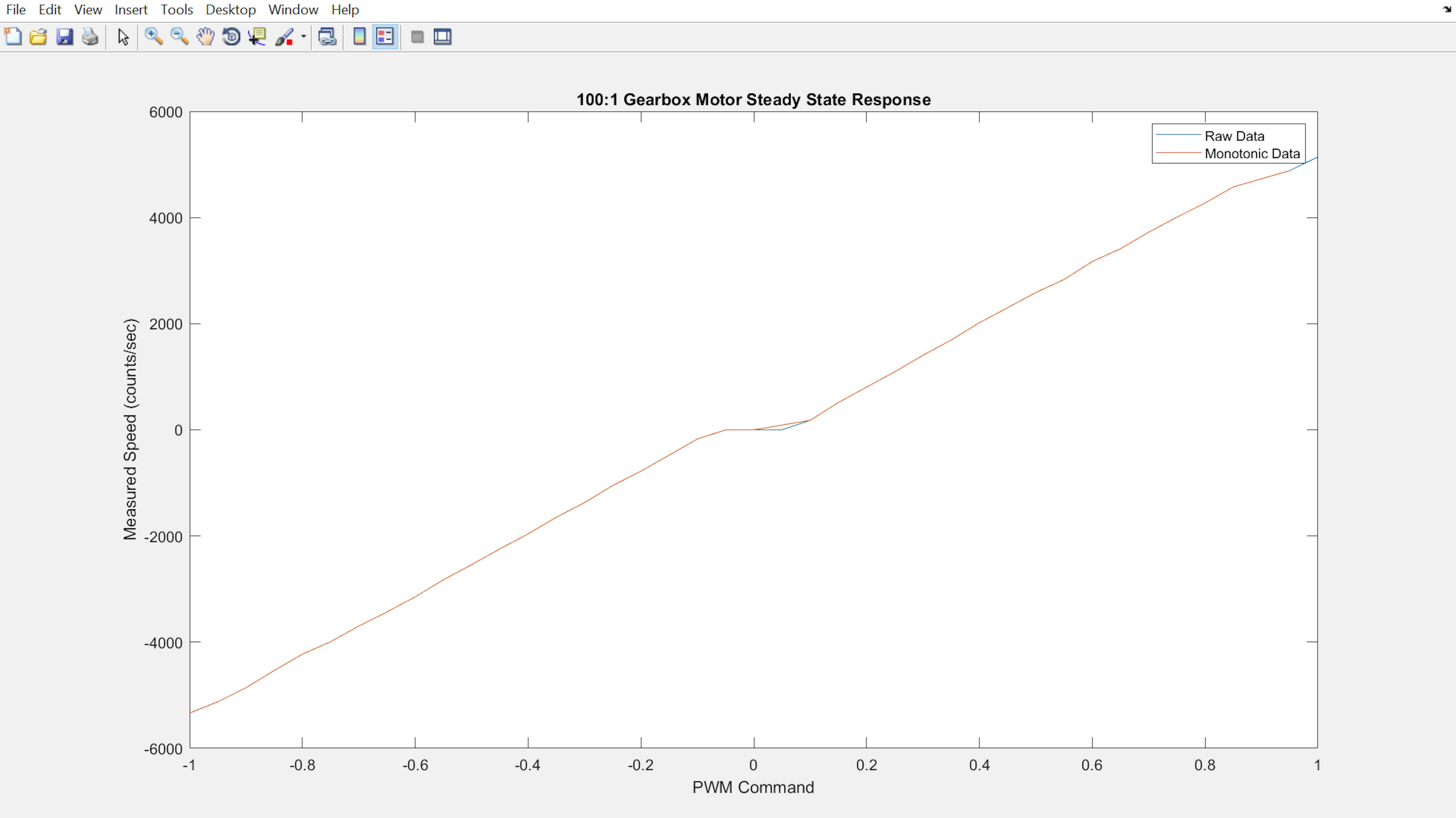
Finally, delete all device objects to release the MKR1000 board to be used in other processes. Add the following section at the end of your live script:
6. Delete device objects
clear a dcm carrier enc
SAVING AND RERUNNING SCRIPTS
You now have a fully functional live script that automatically performs a series of measurements, post-processes those measurements, saves the experimental data to disk, and plots the results. You may want to repeat this analysis multiple times, for the same motor or perhaps other DC motors. You can save your live script as a .mlx file so that you can run it again later or share it with other MATLAB users. Save your live script as myMotorCharacterization.mlx. A .mlx file contains not only your code and text annotations, but also any numeric or graphical results that were displayed in the output column. Thus, your live script is an active report of your analysis and results. Recall that you can run your live script in its entirety using the Run button in the Live Editor window:

You can also run the live script directly in the Command Window using its name as the command. Try running your live script:
>> myMotorCharacterization
CREATING MATLAB FUNCTIONS
Look at your Workspace. Which of the existing variables are useful to you? Which variables are intermediate values from your live script that you no longer need?
You can compartmentalize parts of your MATLAB program into functions, so that the intermediate calculations are hidden and you only need to manage inputs and outputs.
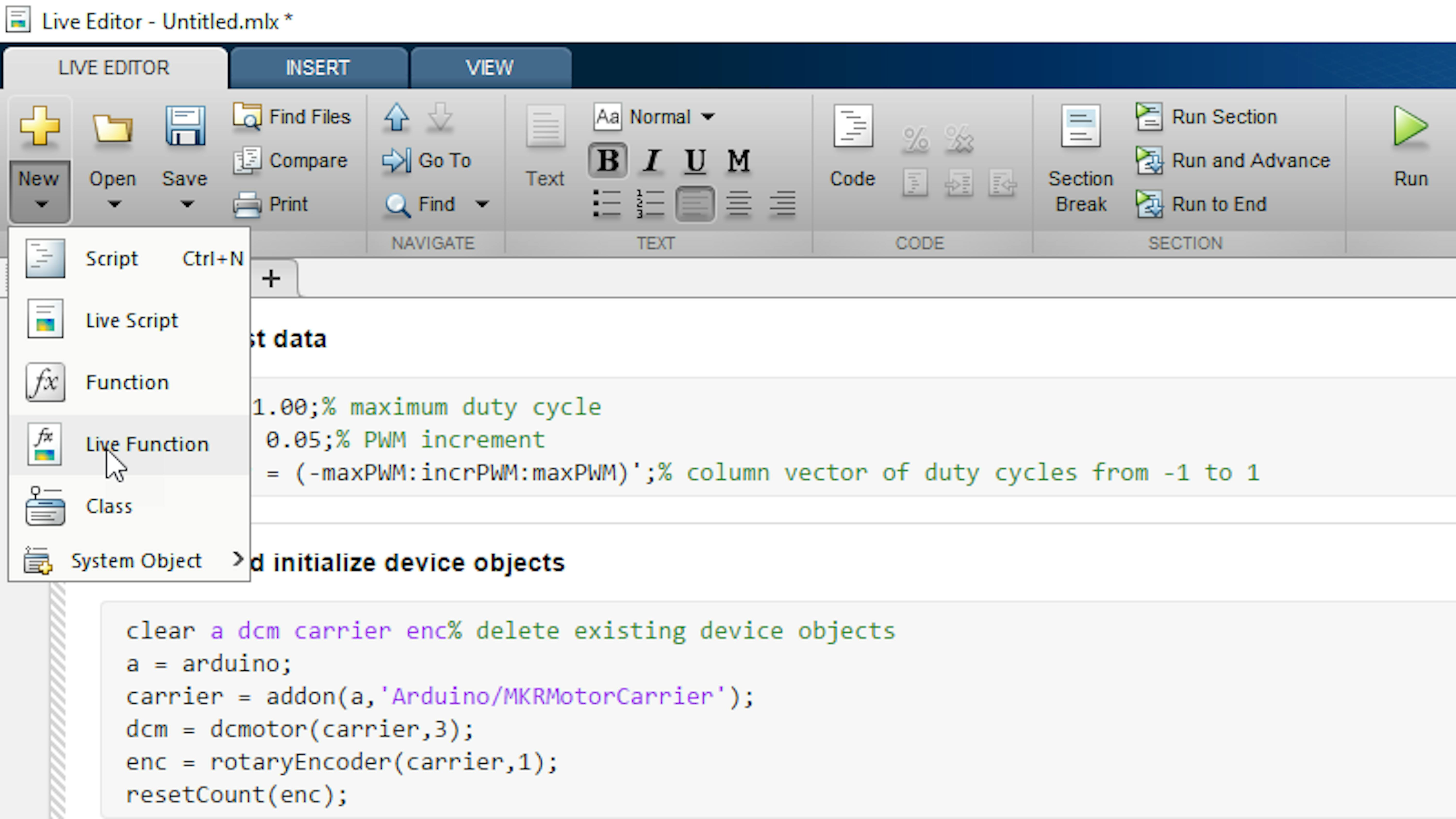
Looking at your live script, the first two sections are specific to this DC motor, encoder, and test case (PWMcmdRaw). The following three sections (measure raw motor speed for each PWM command, post-process and save data, and graph raw and post-processed data) can be generalized for any DC motor, encoder, and test case. Let's create a MATLAB function for that code. Start in the Live Editor window by clicking New>Live Function.
Next, you need to determine what the inputs and outputs to your function are. Section 3 of your live script requires the test vector PWMcmdRaw, the DC motor object dcm, and the encoder object enc.
The next line of code is an example of a possible function header. Place the inputs in parentheses ( () ) with the three variables listed above:
function z = Untitled(PWMcmdRaw,dcm,enc)Now consider what variables you want to access from the motor characterization algorithm. The only meaningful variables created in these sections are PWMcmdMono and speedMono. In the function header, list these two variables as outputs in square brackets ([ ]).
function [PWMcmdMono,speedMono] = Untitled(PWMcmdRaw,dcm,enc)
Finally, let's name the function so that we know how to call it in MATLAB code. Replace the function name with myMotorFunction:
**function** [PWMcmdMono,speedMono] = myMotorFunction(PWMcmdRaw,dcm,enc)Now let's fill in the algorithm. Cut and paste sections 3, 4, and 5 from your live script to your live function, between the function header and the end keyword.
**function** [PWMcmdMono,speedMono] = myMotorFunction (PWMcmdRaw,dcm,enc)
3. Measure raw motor speed for each PWM command
speedRaw = zeros(size(PWMcmdRaw));% Preallocate vector for speed measurements

dcm.DutyCycle = 0;

start(dcm)% turn on motor

**for** ii = 1:length(PWMcmdRaw)

> resetCount(enc);

> startCount = readCount(enc);

> tic;

> dcm.DutyCycle = PWMcmdRaw(ii);

> start(dcm)% turn on motor

> pause(1)% wait for steady state

> stop(dcm);% turn off motor

> dt = toc;

> endCount = readCount(enc);

> speedRaw(ii) = (endCount - startCount) / dt;% calculate speed (cts/s)

> pause(1);

**end**

stop(dcm)% turn off motor

dcm.DutyCycle = 0;
4. Post-process and save data
idx = (diff(speedRaw) > 0);% find indices where vector is increasing

speedMono = speedRaw(idx);% Keep only increasing values of speed

PWMcmdMono = PWMcmdRaw(idx);% Keep only corresponding PWM values

PWMcmdMono(speedMono == 0) = 0;% enforce zero power for zero speed

save motorResponse PWMcmdMono speedMono% save post-processed measurements
5. Graph raw and post-processed data
plot(PWMcmdRaw,speedRaw)% raw speed measurements

hold on

plot(PWMcmdMono,speedMono)% non-monotonic measurements filtered out

title('100:1 Gearbox Motor Steady State Response')

xlabel('PWM Command')

ylabel('Measured Speed (counts/sec)')

legend('Raw Data','Monotonic Data')

**end**
Save the file as myMotorFunction.mlx. Now you have a working MATLAB function that you can call from any MATLAB code environment. Let's try calling it from your live script. In the empty section of your live script, enter the call to your function:
1. Create test data
maxPWM = 1.00;% maximum duty cycle
incrPWM = 0.05;% PWM increment
PWMcmdRaw = (-maxPWM:incrPWM:maxPWM)';% column vector of duty cycles from -1 to
1
2. Create and initialize device objects
clear a dcm carrier enc% delete existing device object
a = arduino;
carrier = addon(a,'Arduino/MKRMotorCarrier');
dcm = dcmotor(carrier,3);
enc = rotaryEncoder(carrier,1);
resetCount(enc);
3-5. Call motor characterization function
[PWMcmdMono,speedMono] = myMotorFunction(PWMcmdRaw,dcm,enc);
Now run your live script and ensure it still works as before.
To further understand the benefits of using MATLAB functions, clear your Workspace in the Command Window , and run your live script again.
>> clear
>> myMotorCharacterization
Examine your Workspace. The list of variables should be more concise now. There is one more thing you may want to generalize in this function, and that is the name of the MAT-File that we use in the save command. As of now, the analysis data gets saved to the same MAT-File, motorResponse.mat, every time you call the function. This is not very useful if you want to characterize multiple DC motors. Let's add a new input to the function for the file name. In the live function, add the new input as shown below:
function [PWMcmdMono,speedMono] = myMotorFunction(PWMcmdRaw,dcm,enc,filename)
Now let's use the new input in the save command. Rewrite the save command as follows :
save(filename,'PWMcmdMono','speedMono')% save post-processed measurements Finally, we need to modify the function call, since the function header has changed. In the live script, change the function call as follows:
[PWMcmdMono,speedMono] = myMotorFunction(PWMcmdRaw,dcm,enc,'motorResponse');
Now you can save the analysis data to any MAT-file you want each time you call myMotorFunction. Try calling your live script once more:
>> myMotorCharacterization2.3
Simulink getting started
MATLAB allows you to perform a whole series of operations on data using code as an interface. Simulink offers a visual programming language (VPL) based on the use of a flow programming paradigm to route data, process it, save it, and send the outcomes to other programs, to MATLAB scripts, and even Arduino boards.
One of the most exciting features of the Simulink VPL is the possibility of designing programs that could be uploaded to Arduino boards directly from within MATLAB IDE. This section will give you a brief introduction to Simulink and this workflow.
SYSTEM MODELING IN SIMULINK
In this section, you will learn:
- How to create, simulate, and save a Simulink model.
- How to add and remove blocks from a Simulink model.
- How to connect blocks in a block diagram.
- How to label blocks and signals.
- How to set block parameter values.
- How to visualize simulation data in the Simulink environment.
- How to set the sampling rate of block in a Simulink model.
- How to add block hierarchy to a Simulink model using subsystems.
You now have experimental data that defines the relationship between the 100:1 gearhead DC motor's speed and the applied voltage via the PWM command. Let's begin by designing a motor control system that takes the user's desired speed as input and determines the necessary PWM command to achieve that speed. You will use Simulink to model and simulate this system, and in the next section you will run your Simulink model directly on the MKR1000 board. Let's visualize how this control system will work:
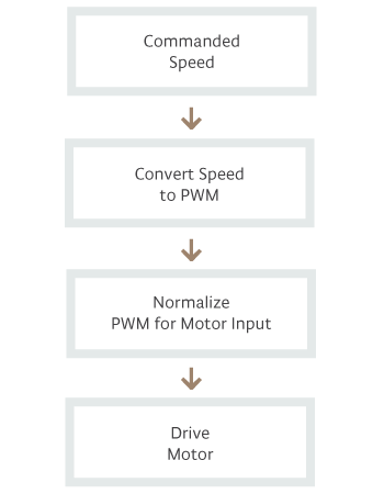
In this diagram, the blocks represent some functionality or process and the arrows represent data flow. The directionality of the arrows indicate which process generates the data and where the data is used. Simulink enables you to create your algorithm as a block diagram and execute it over an interval of time.
CREATING A NEW SIMULINK MODEL
Let's start up the Simulink environment. In the MATLAB desktop, click the Simulink button:
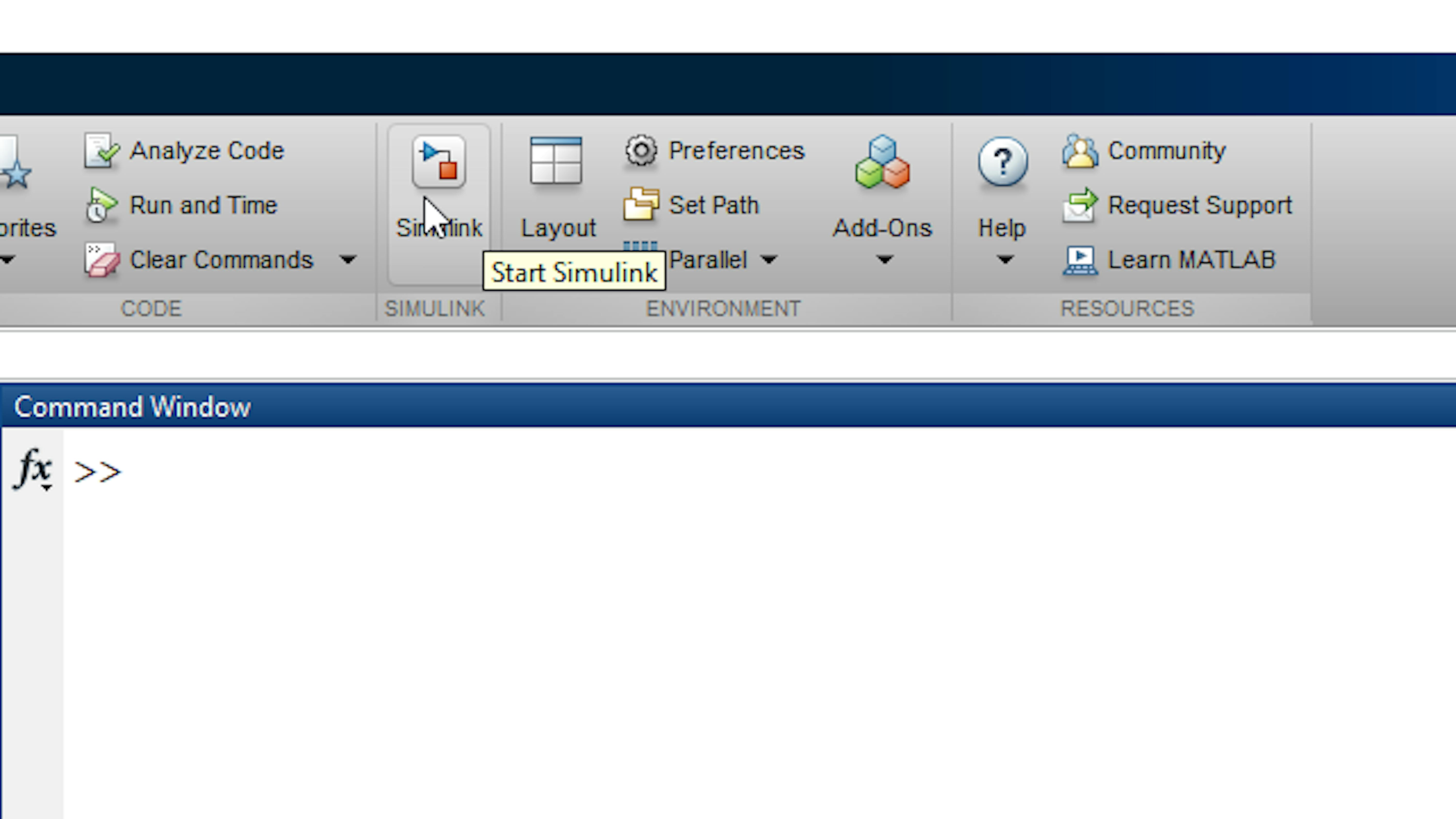
In the Simulink Start Page window, click Blank Model to open the Simulink Editor:
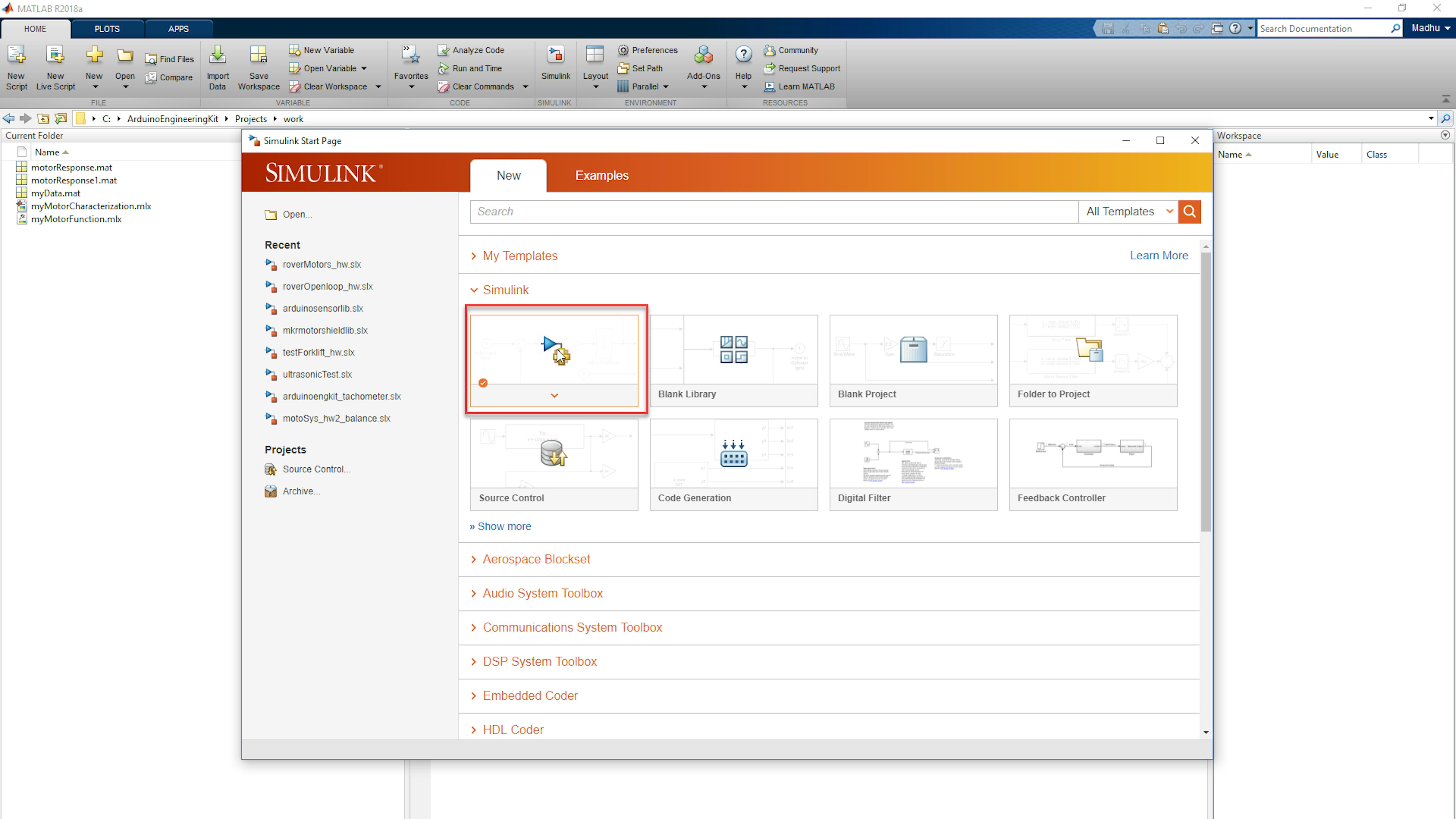

BLOCKS AND SIGNALS
Now let's add some blocks to the model canvas. You can find all the built-in Simulink blocks by using the Simulink Library Browser. Open the Simulink Library Browser by clicking the Library Browser button in the toolstrip, as shown below:
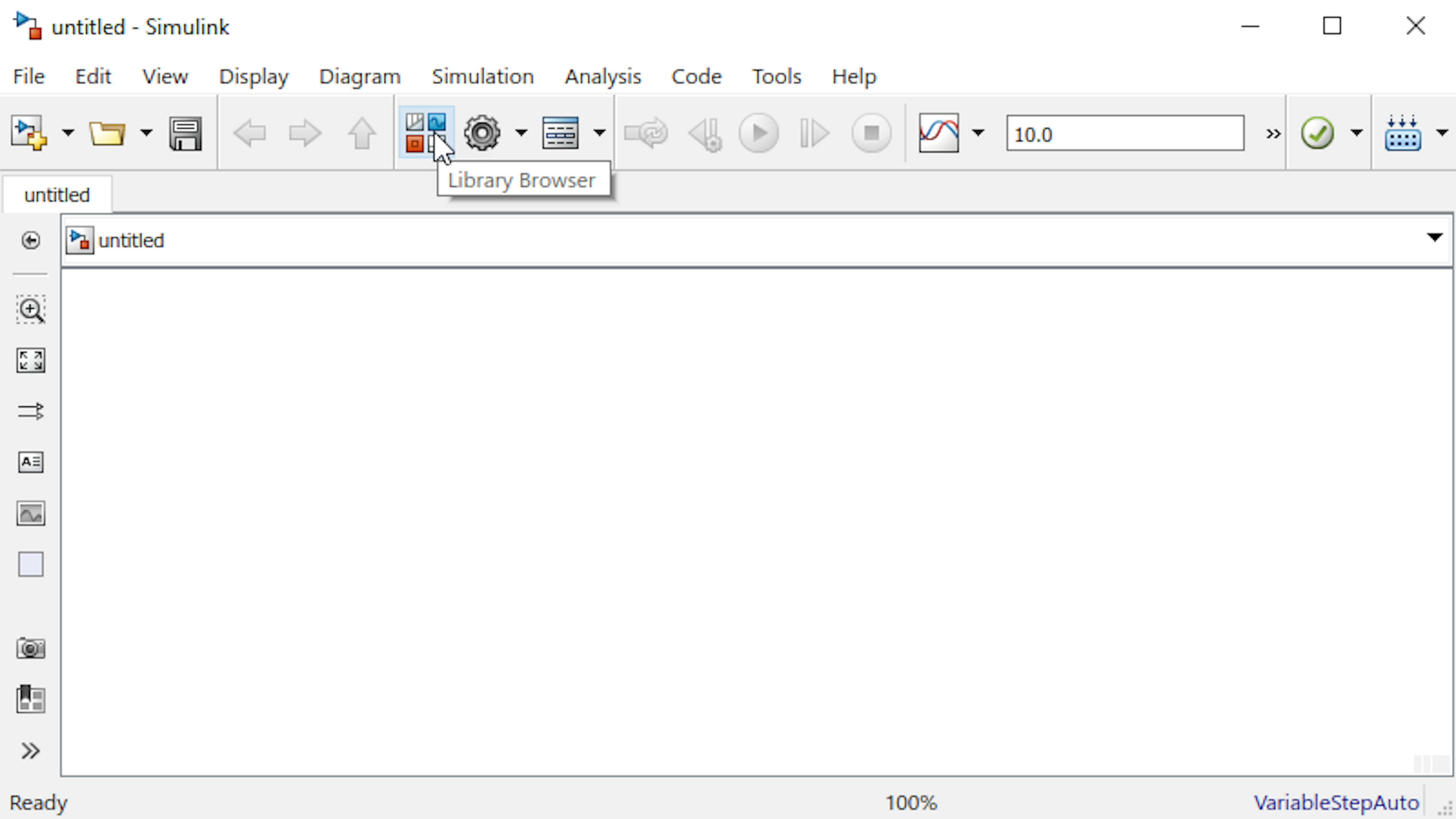
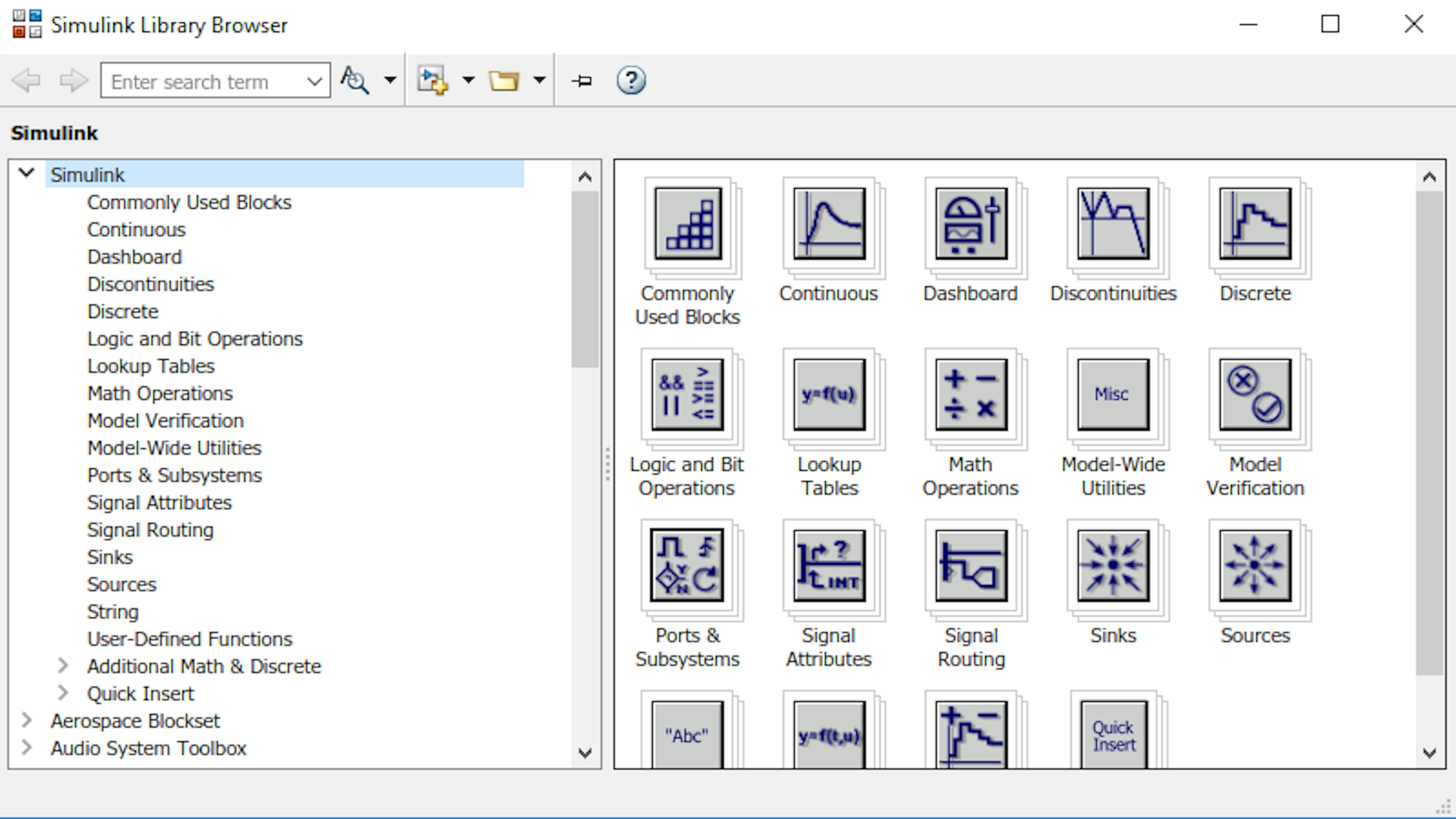
In the left panel, the Simulink Library Browser shows a list of the add-on products, and within each a number of libraries are made available. Throughout the projects in the Arduino Engineering kit, you will use blocks from several libraries, including basic Simulink blocks and Simulink Support Package for Arduino Hardware. Examine the Sources library under Simulink.
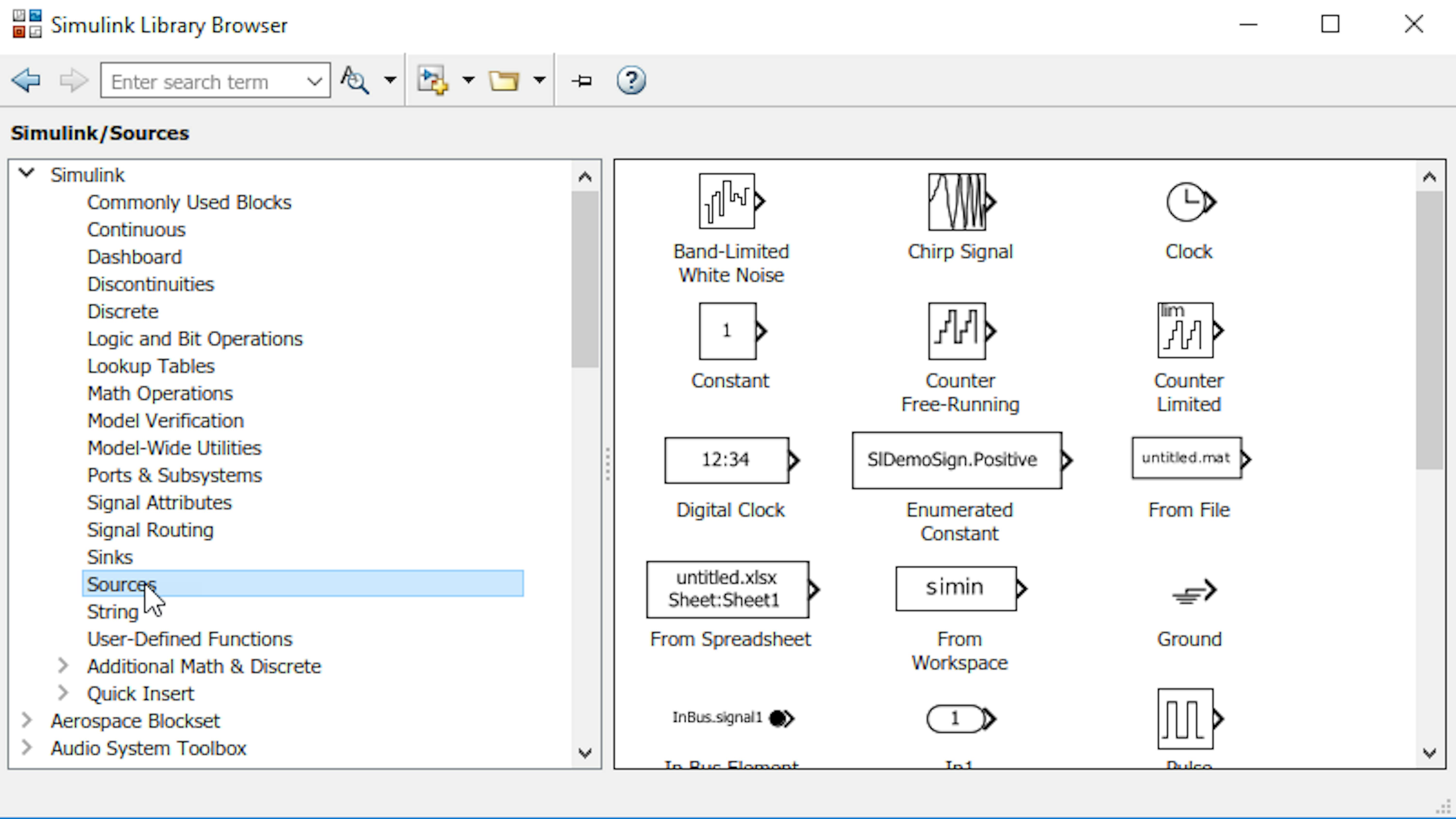
These blocks function as inputs to a Simulink block diagram. Notice that they all have triangular ports on their right sides. These are called outports and allow you to connect signals at their origin. To test your motor control system, you will use a sine wave to simulate the speed input. Locate the Sine Wave block and drag it from the Simulink Library Browser window to the Simulink Editor window.
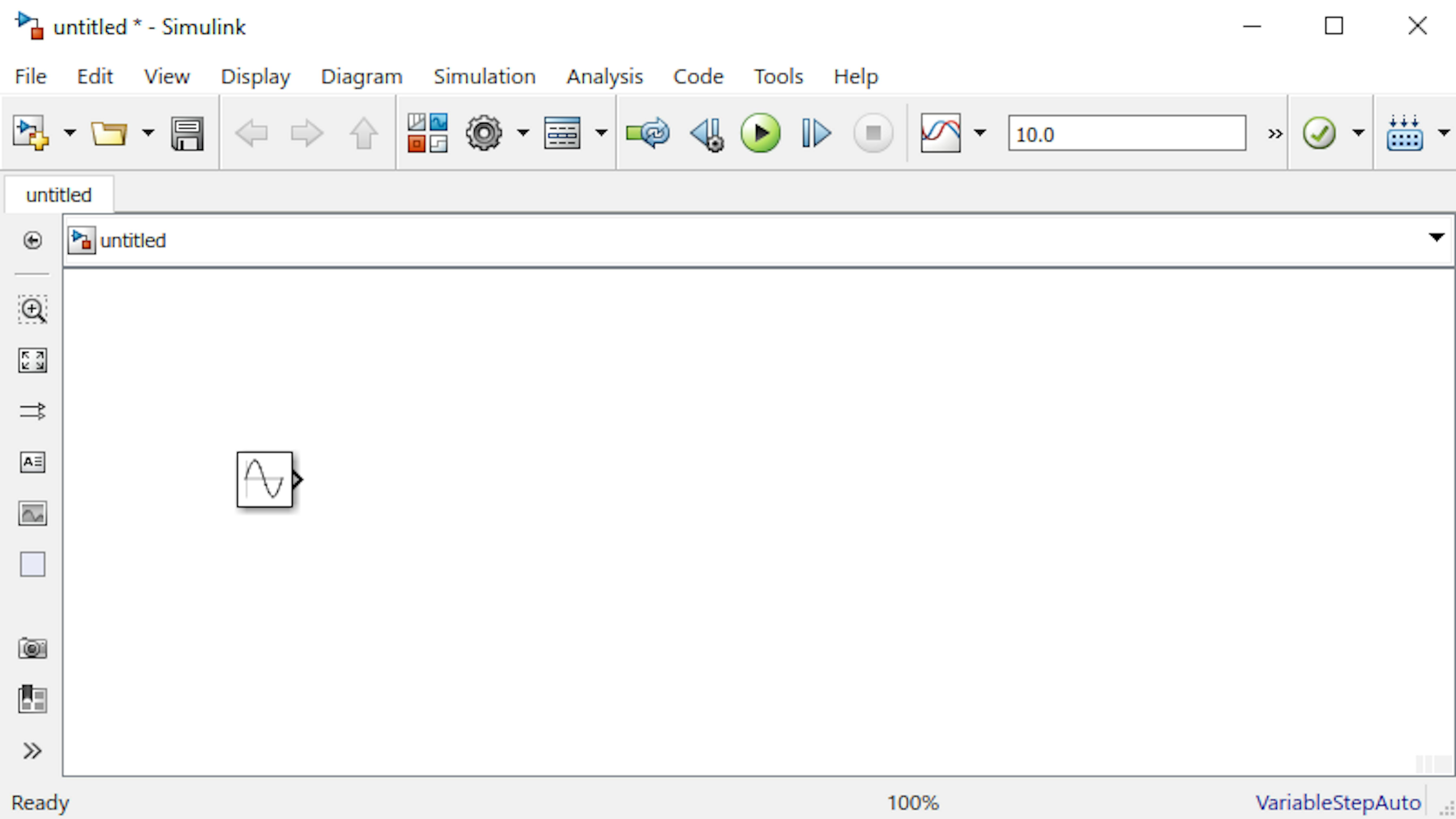
Next you need to convert the user's speed signal coming from the Sine Wave block into a PWM signal between -1 and 1. To do this, use a lookup table, which uses interpolation among known data points to determine an output value for an arbitrary input value. We'll discuss this in more detail shortly. Locate the 1-D Lookup Table block in Simulink > Lookup Tables and drag it into the Simulink Editor window.

Note: You can zoom and pan in the Simulink Editor using the scroll wheel on your mouse. To zoom to all the content in the model, press the spacebar on your keyboard.
The Lookup Table will output PWM command values between -1 and 1. Ultimately, you will communicate the magnitude of the duty cycle to the DC motor hardware using 8-bit integers that range from 0 to 255. To prepare for this scaling, you need a Gain block. A Gain block multiplies a Simulink signal by a constant value. Add a Gain block from Simulink > Math Operations:
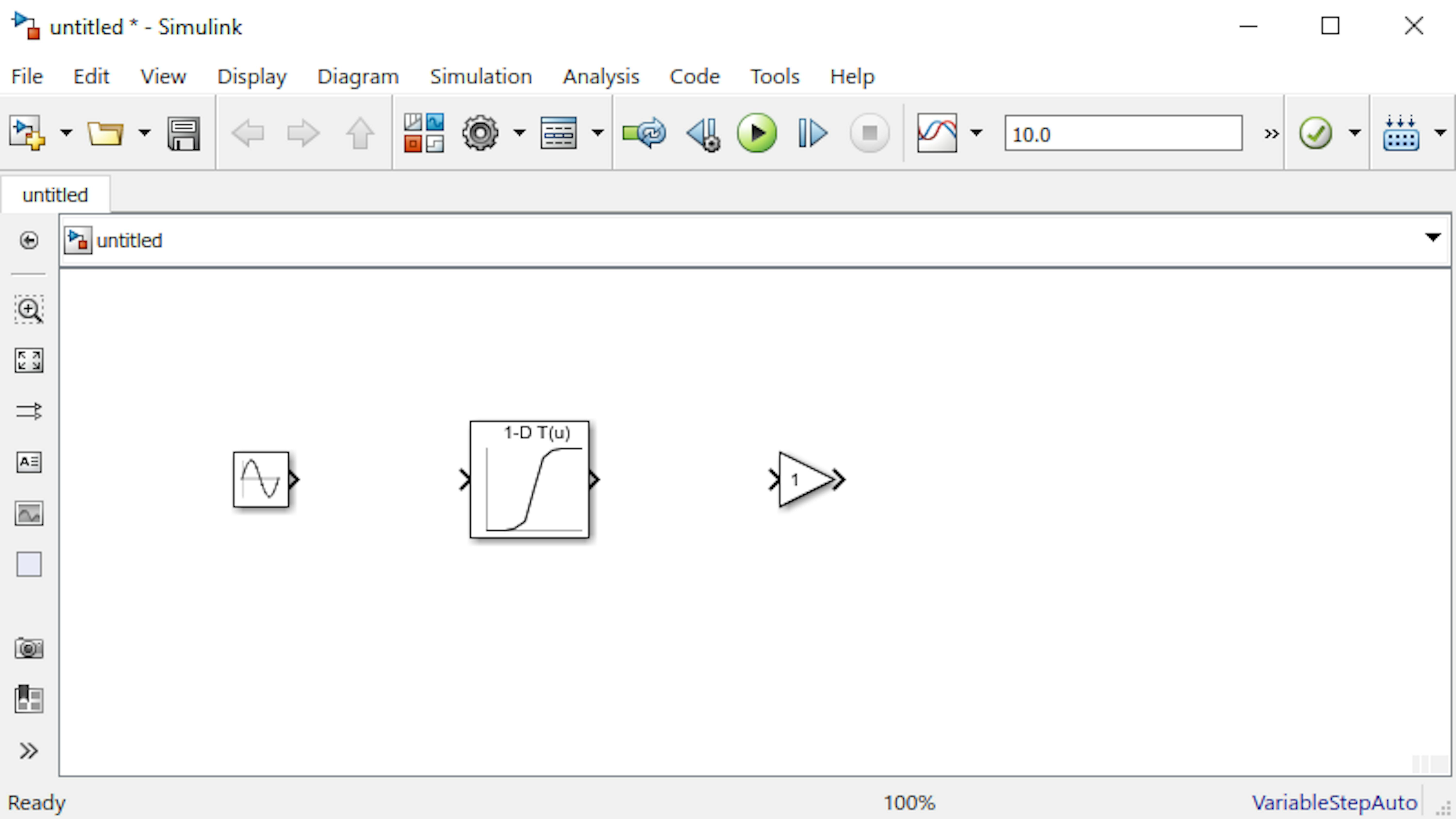
Now let's add a block to visualize the output of the lookup table. Examine the Simulink > Sinks library.
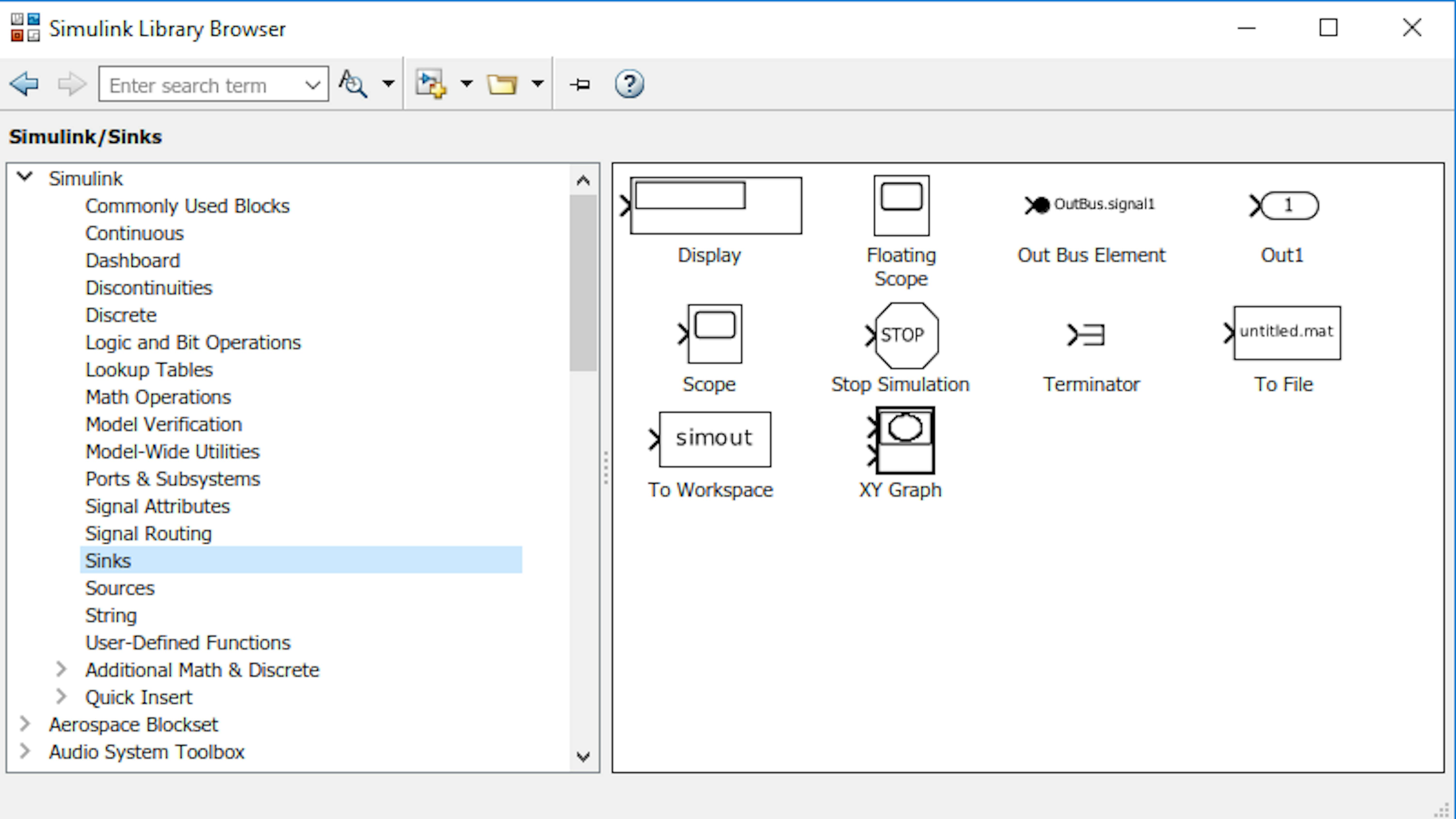
These blocks represent outputs in your block diagram. Notice that these blocks generally have an inward triangular port on their left, known as an inport. Block inports allow you to terminate a signal. Drag a Scope block into your model:
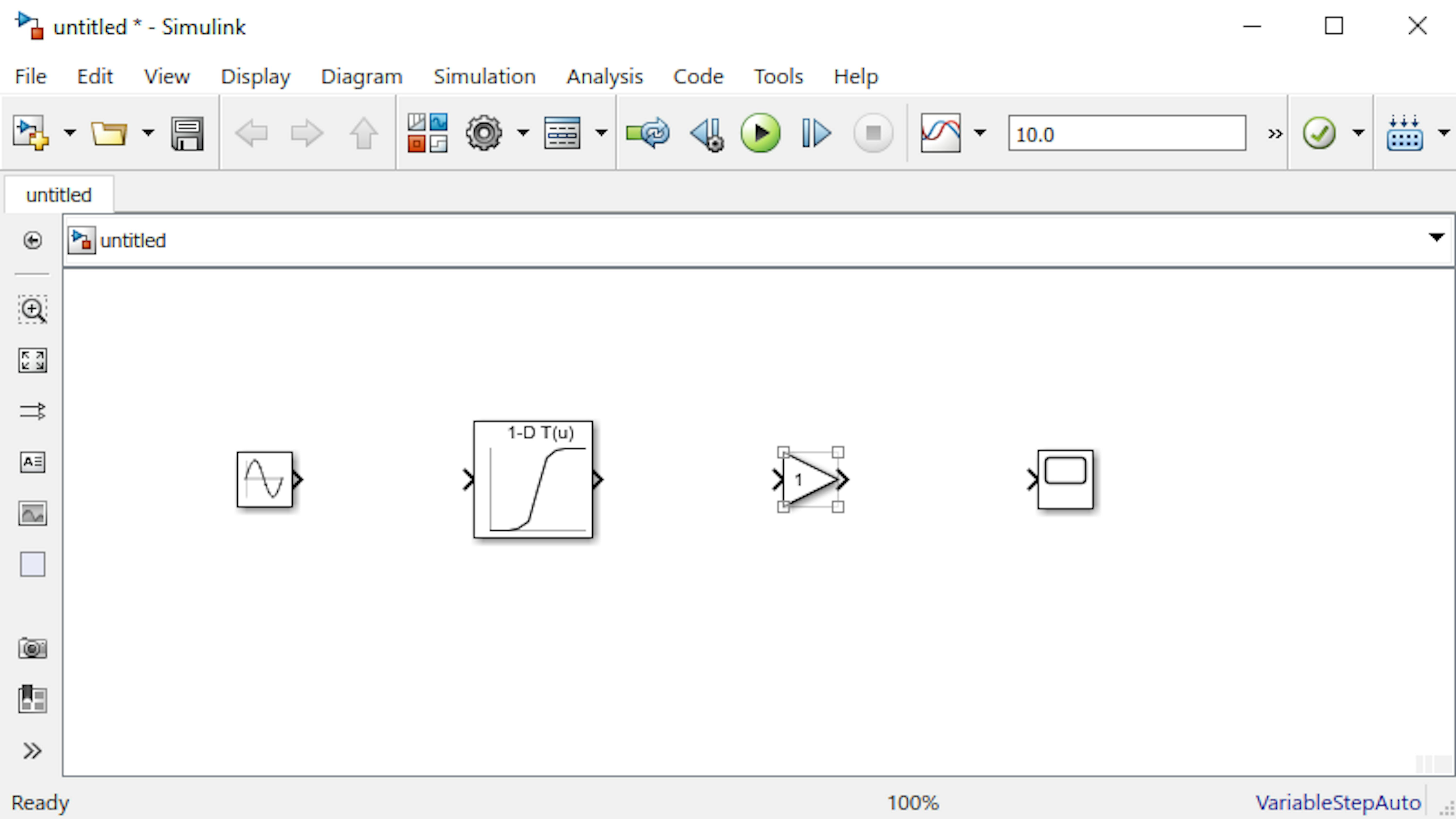
Now you need to connect the blocks using signals. Left click on the outport and drag it to the inport and when the signal line turns solid, you have connected the signal and you can stop the click and drag.
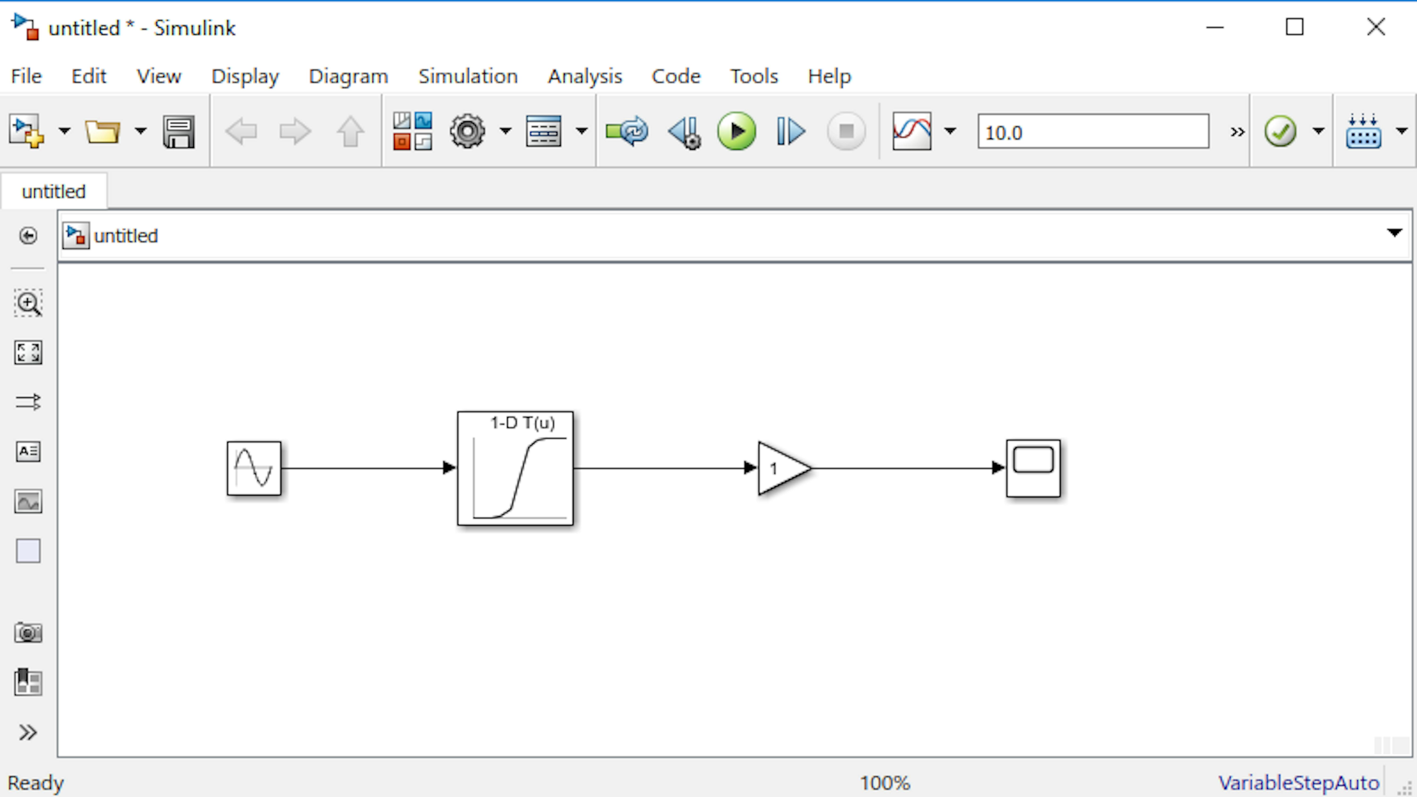
Now let's configure the blocks to perform your specific algorithm. The Sine Wave block needs to generate speed values in counts per second. Examine the range of speeds that you measured for the motor; to do this, look into the data files you generated in the MATLAB section of this chapter by issuing the following commands in the command window:
>> load motorResponse
>> min(speedMono)
>> max(speedMono)
Note: If you did not generate the file motorResponse.mat, run the command >> arduinosetup. Then, configure the MKR1000 as in "Configuring Arduino Libraries" and run the command >> characterizeMotorScript to characterize the motor response. Then run the above commands. Double-click the Sine Wave block to open its block parameter dialog. Configure the sine wave to have an amplitude of 6000, to cover the range of measured speeds. Then click OK:
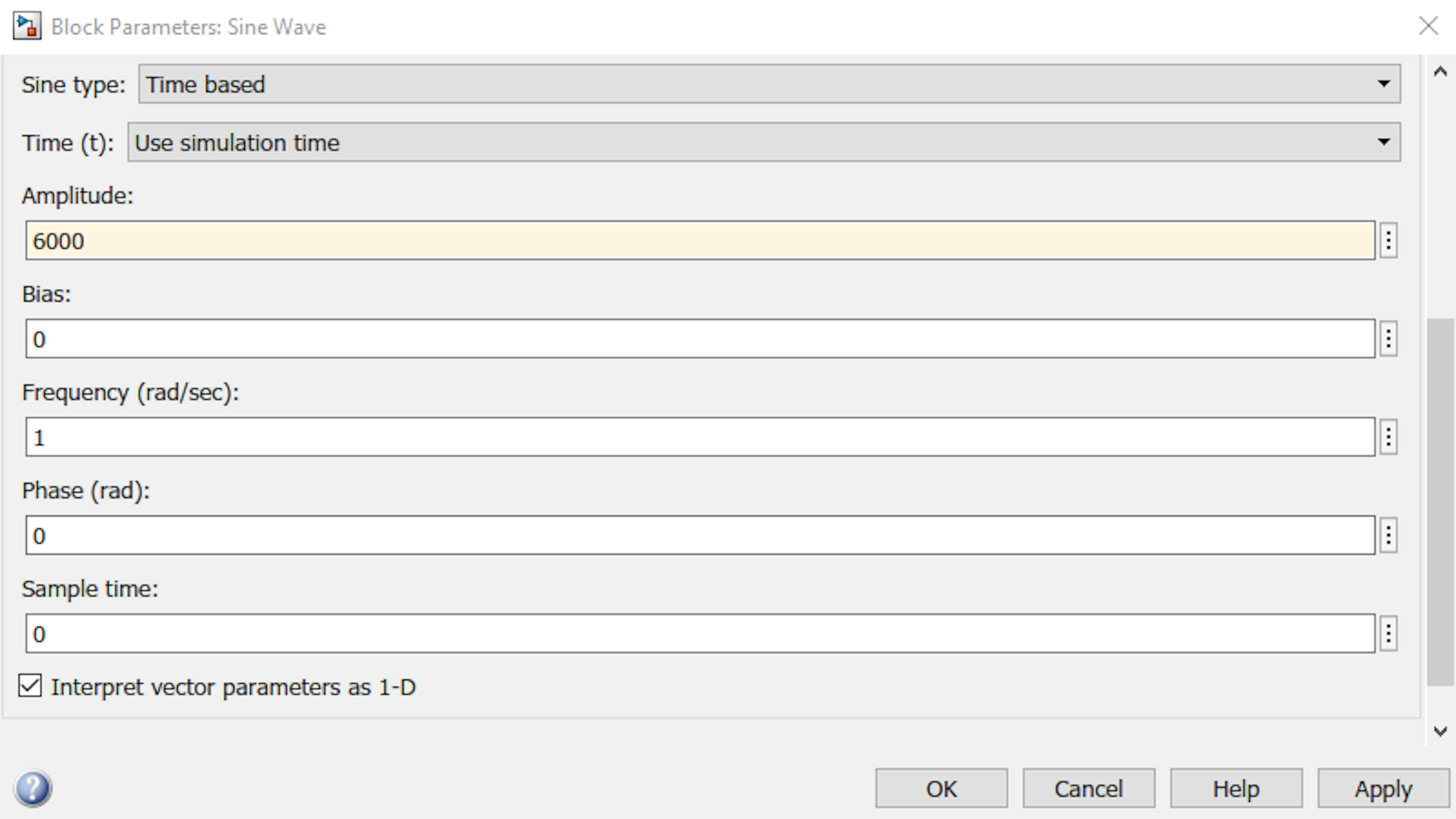
Note: We obtained the value of 6000 empirically; please check whether it also suits you.
Now let's set up the lookup table to map speeds to PWM commands. During simulation, the block will use linear interpolation to estimate the value of the PWM command to achieve an arbitrary speed:
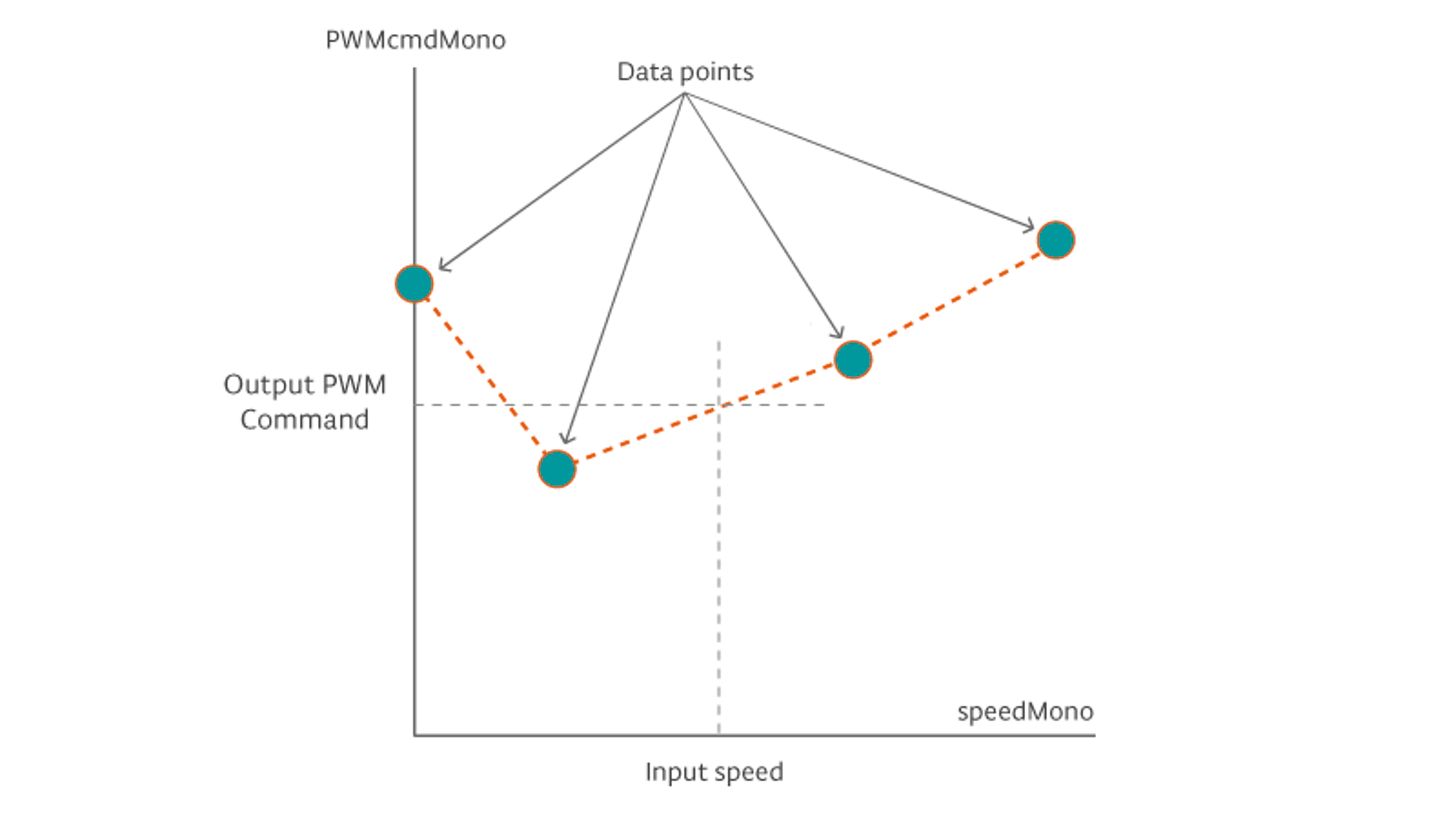
Double-click the 1-D Lookup Table block to open its block parameter dialog. Set Table data to PWMcmdMono and set Breakpoints to speedMono. Then click OK:
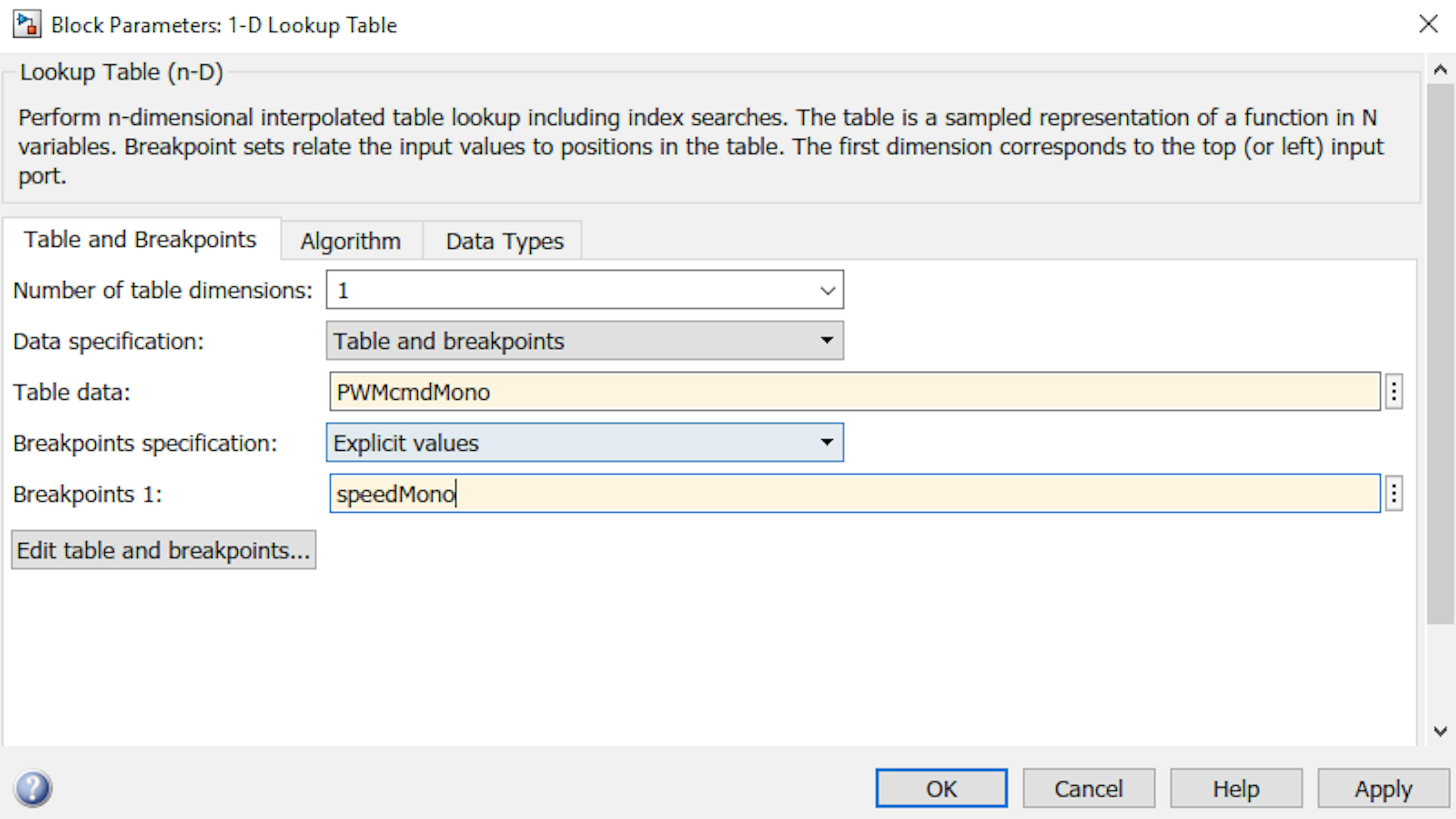
Once you set the lookup table data, the block will show a graph of your lookup table vectors:
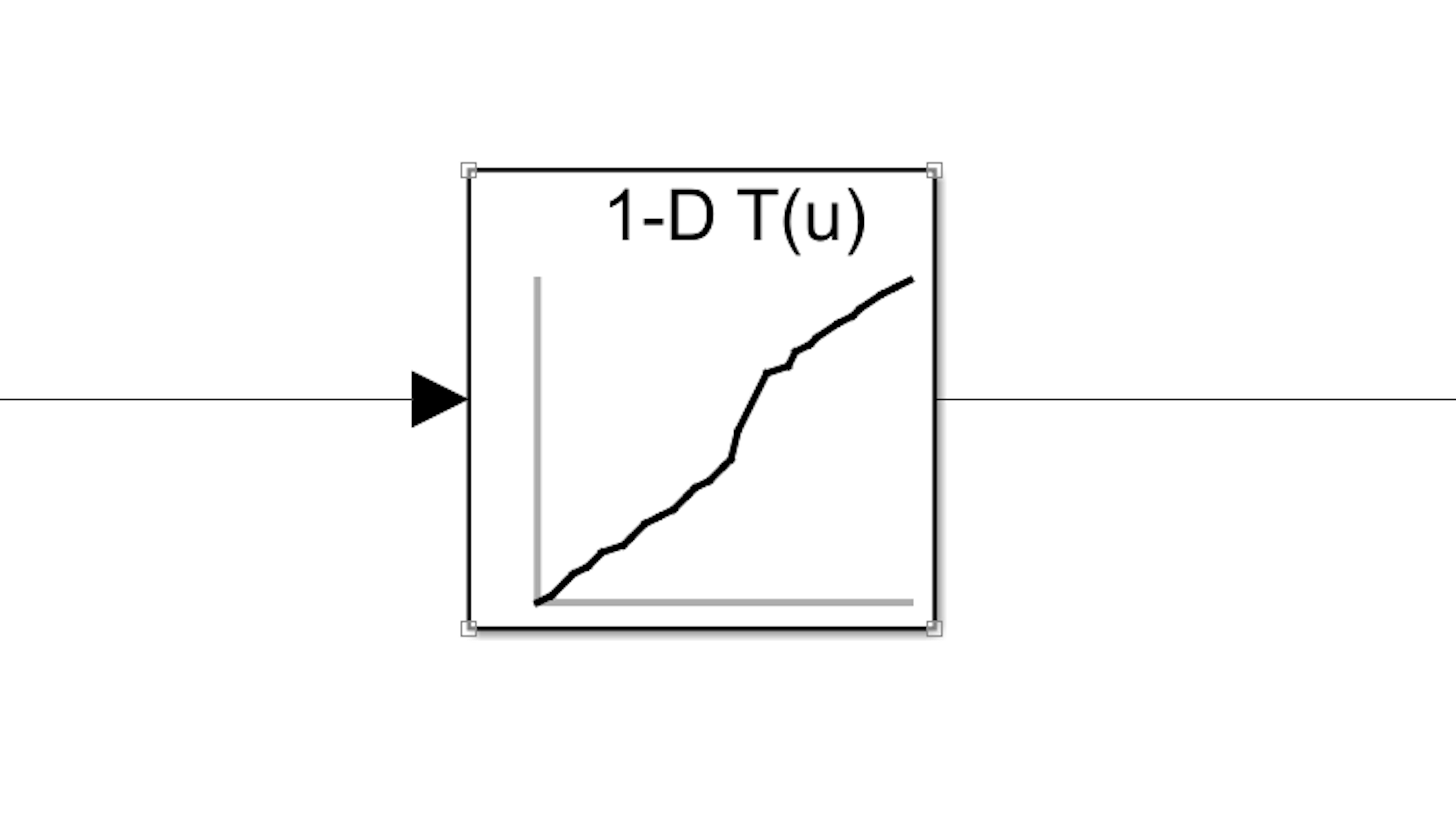
Now let's amplify the PWM duty cycle to cover a range of -255 to 255, to be compatible with the motor driver later. Double-click the Gain block and set Gain to 255. Then click OK:
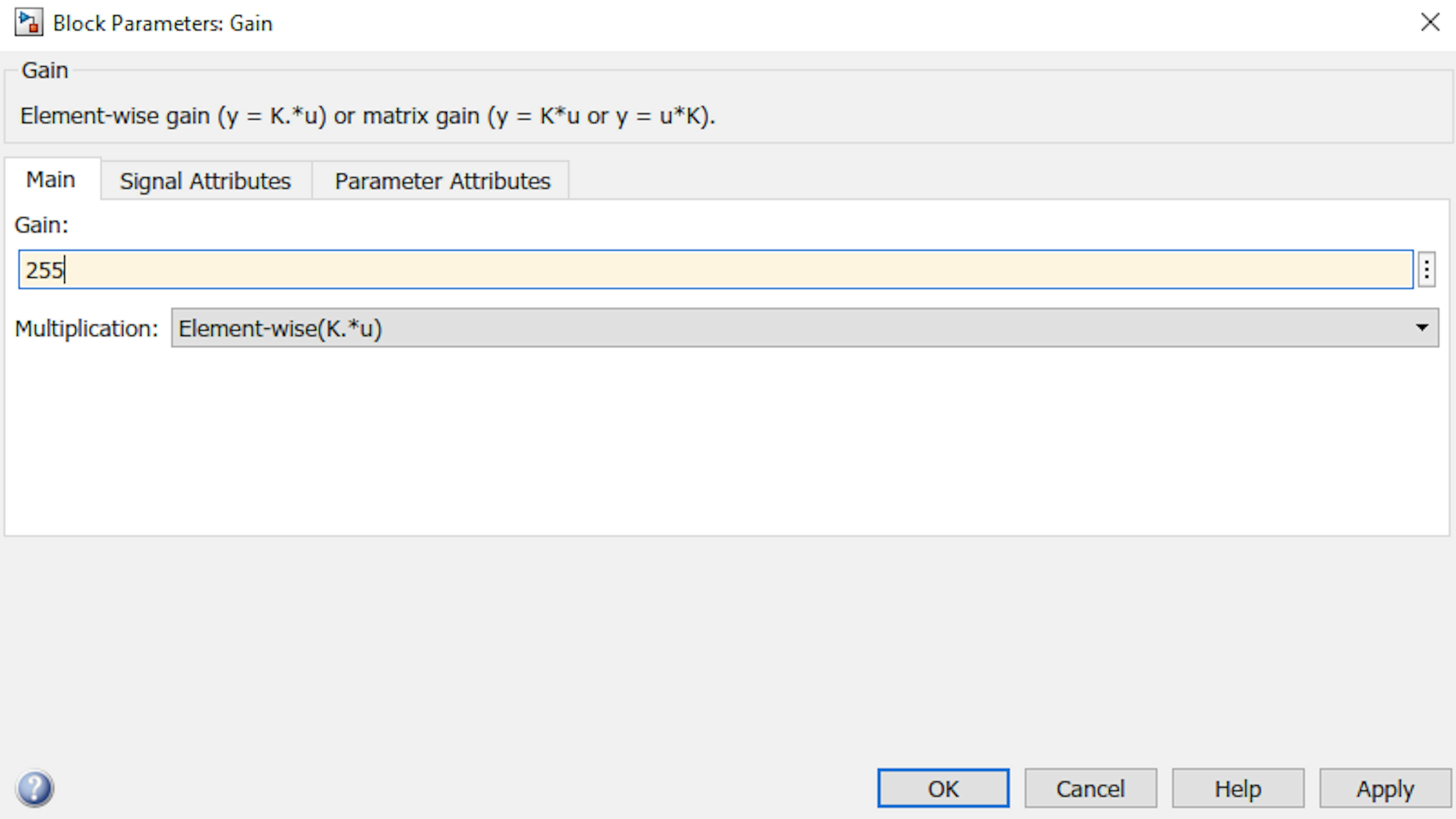
At this point you have finished making a Simulink model capable of generating a signal that you can send later to the MKR board to control the speed of a motor connected to the MKR Motor Carrier.
SIMULATING A MODEL
Let's simulate the algorithm you just created. Click the Run button:
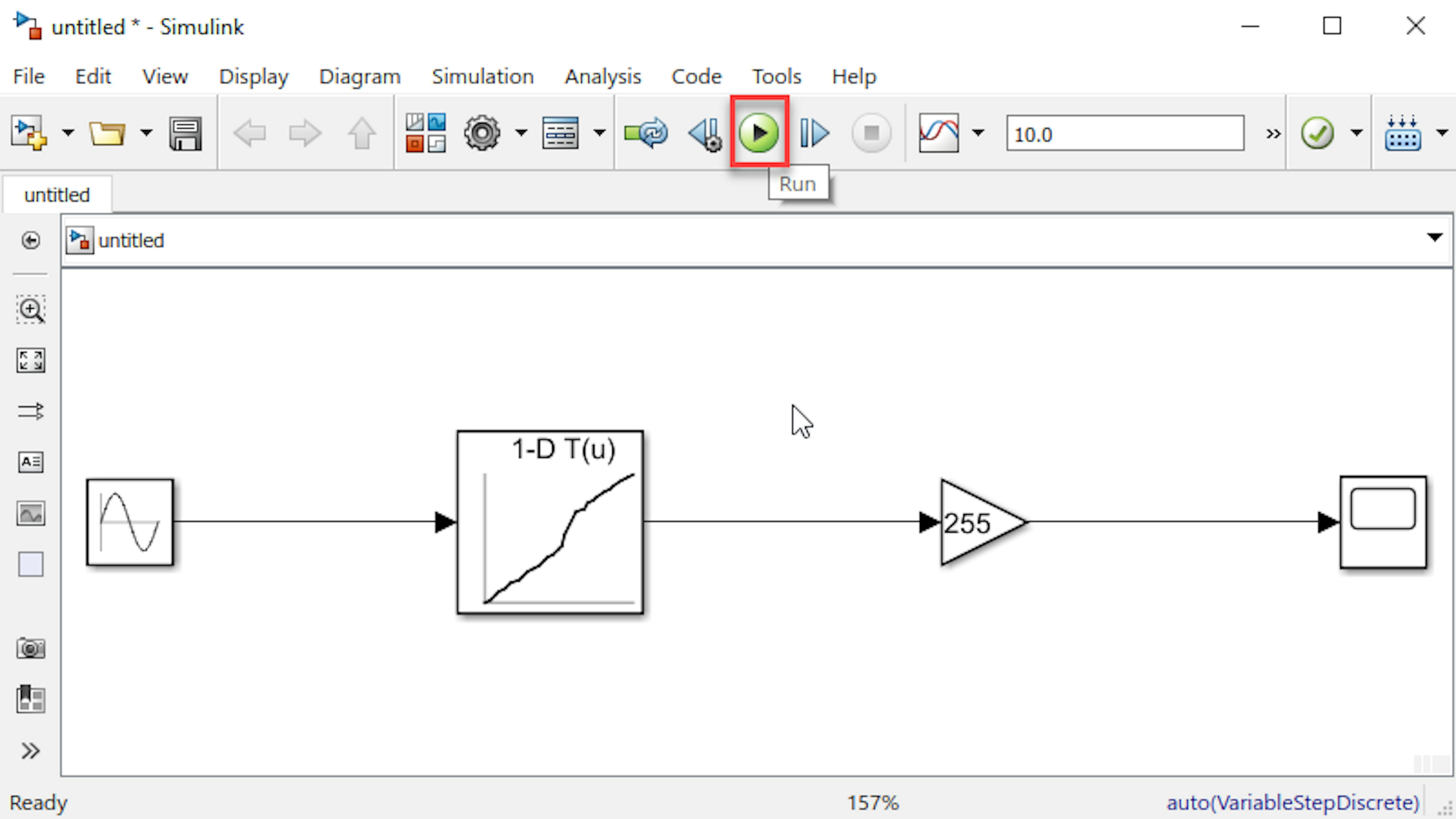
Once the simulation completes, double-click the Scope block to view the scaled PWM values:
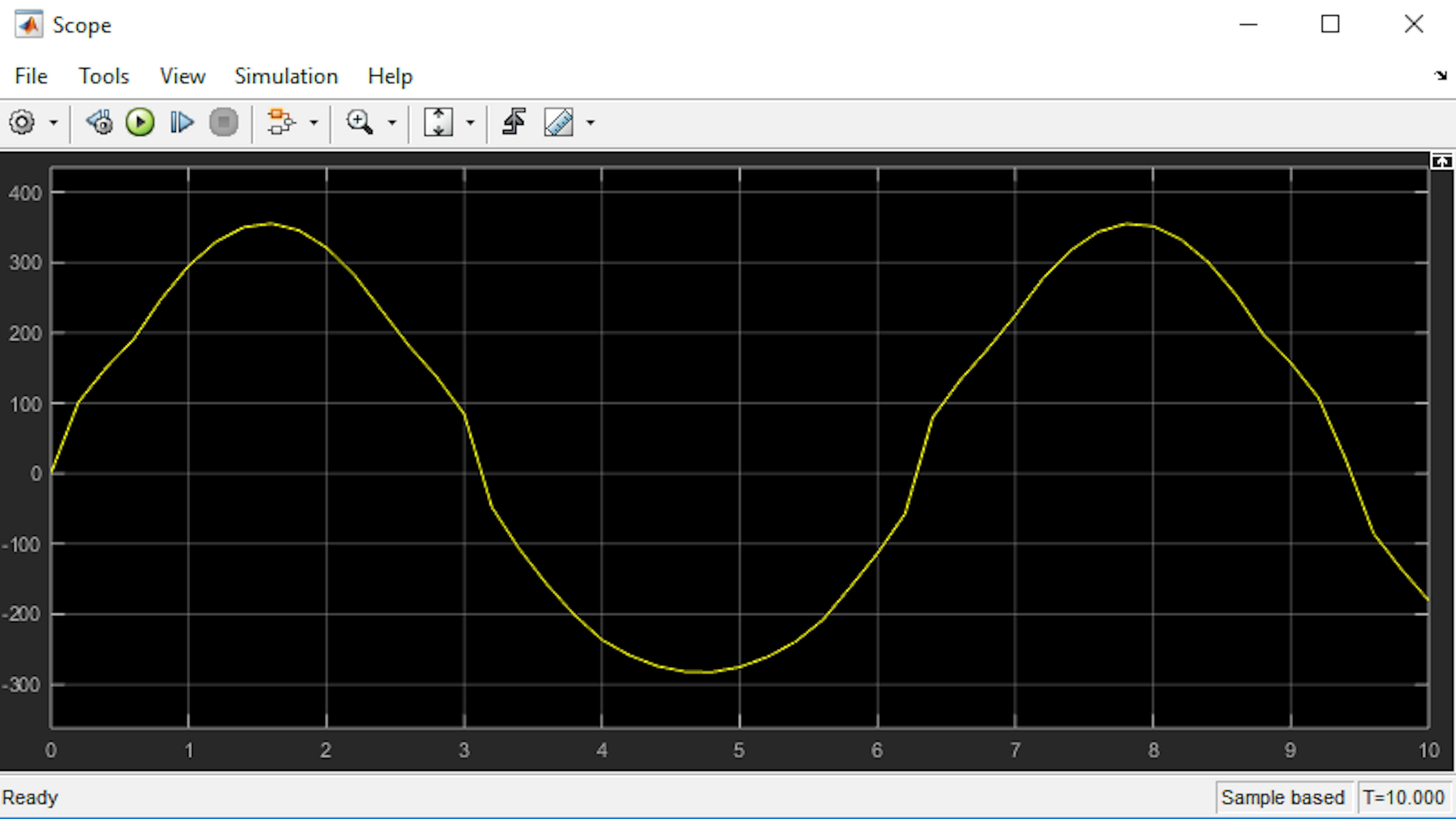
You should expect to see some vertically distorted version of a sine wave when the speed command is converted to respective PWM value. It would be even more informative to simultaneously view the input speed along with the output PWM command. You need to route the speed input signal to the Scope, below the existing import. To do this, you will need to branch the speed input signal. Right click on the speed input signal line and hold down the right mouse button, then drag it to the Scope block. A second import will automatically be created for you:
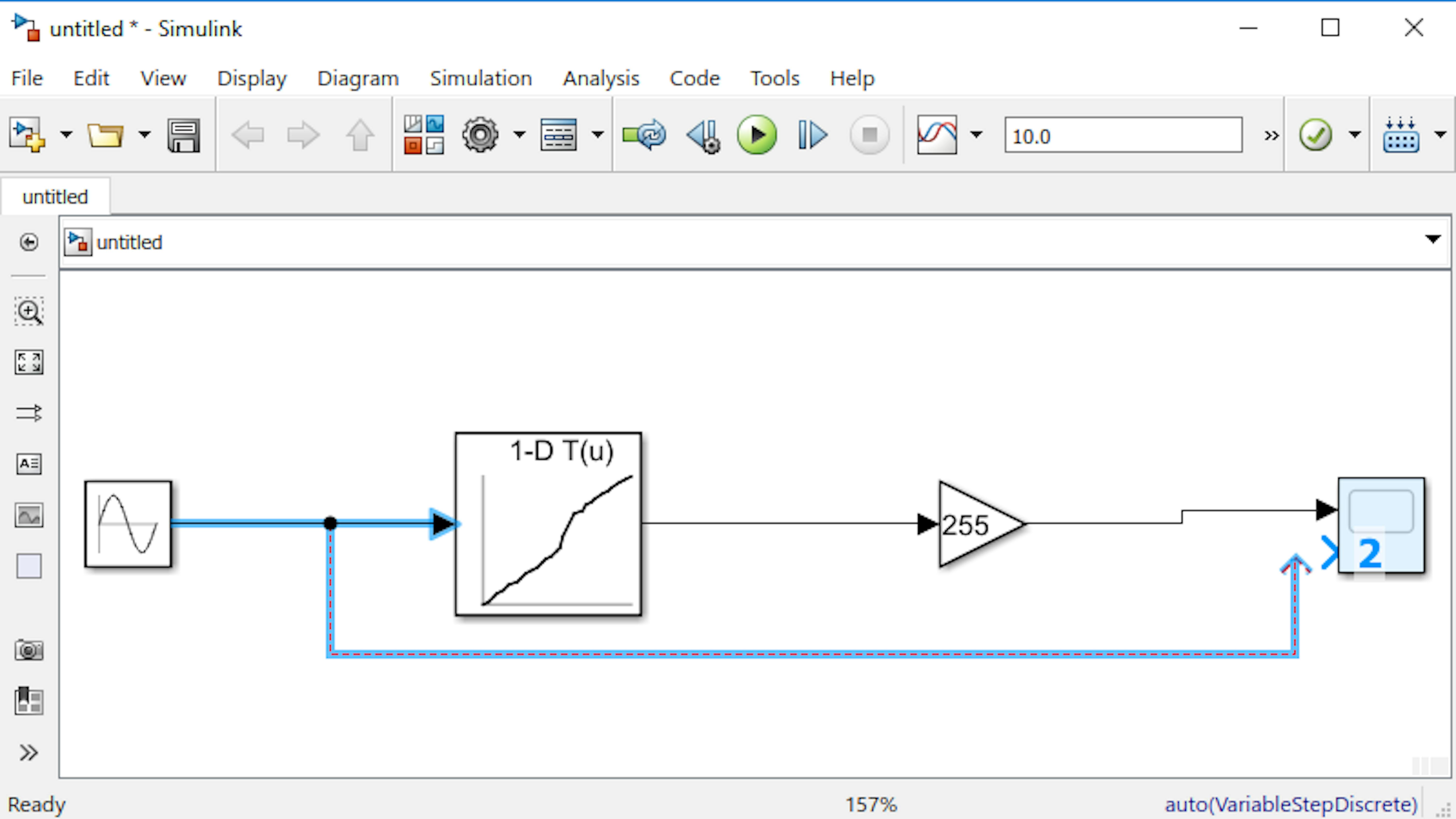
Go to the Scope window, and click View > Layout, and set the axes layout to be 2 x 1, as shown in the image below:
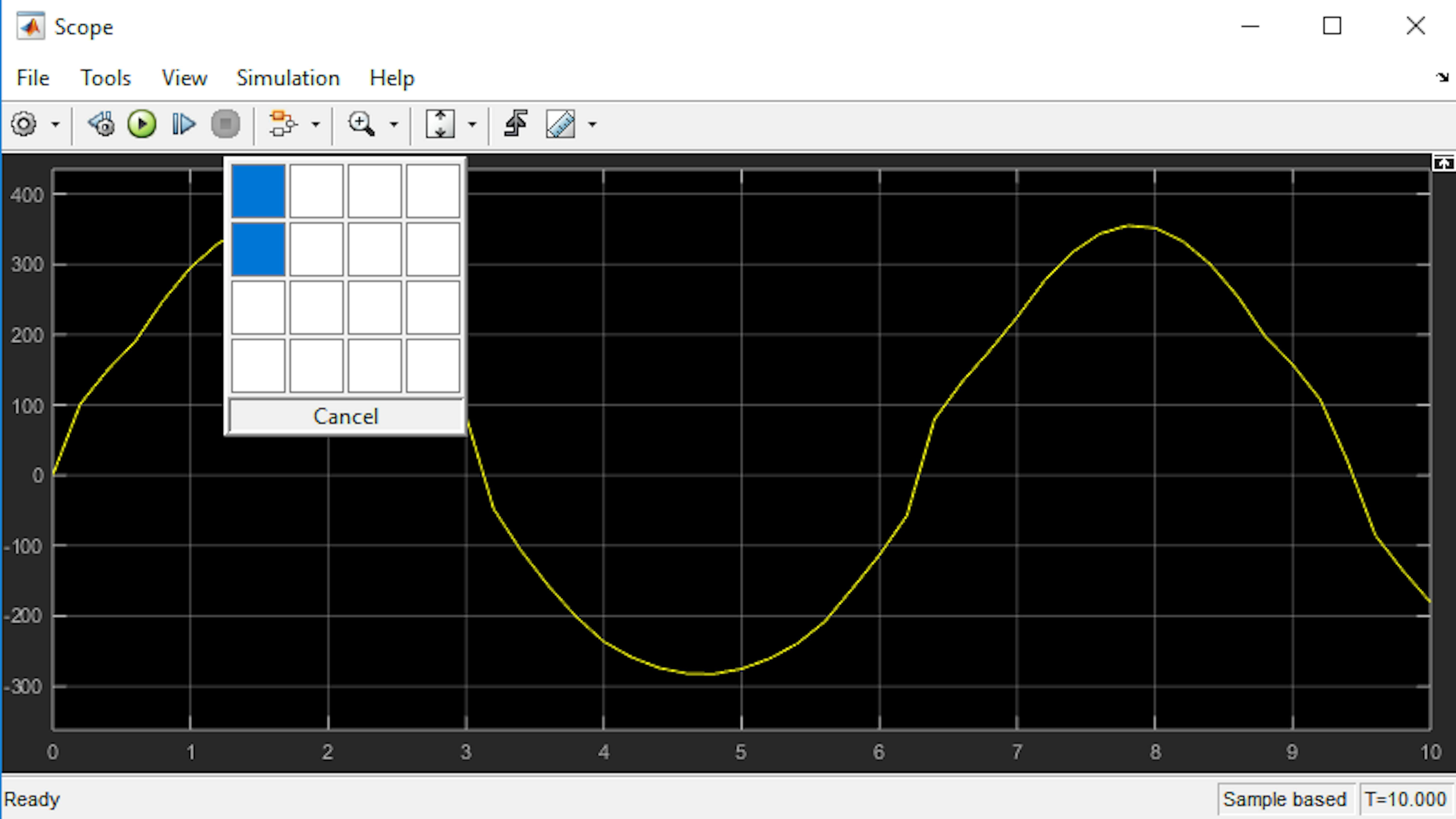
Return to the Simulink Editor window:
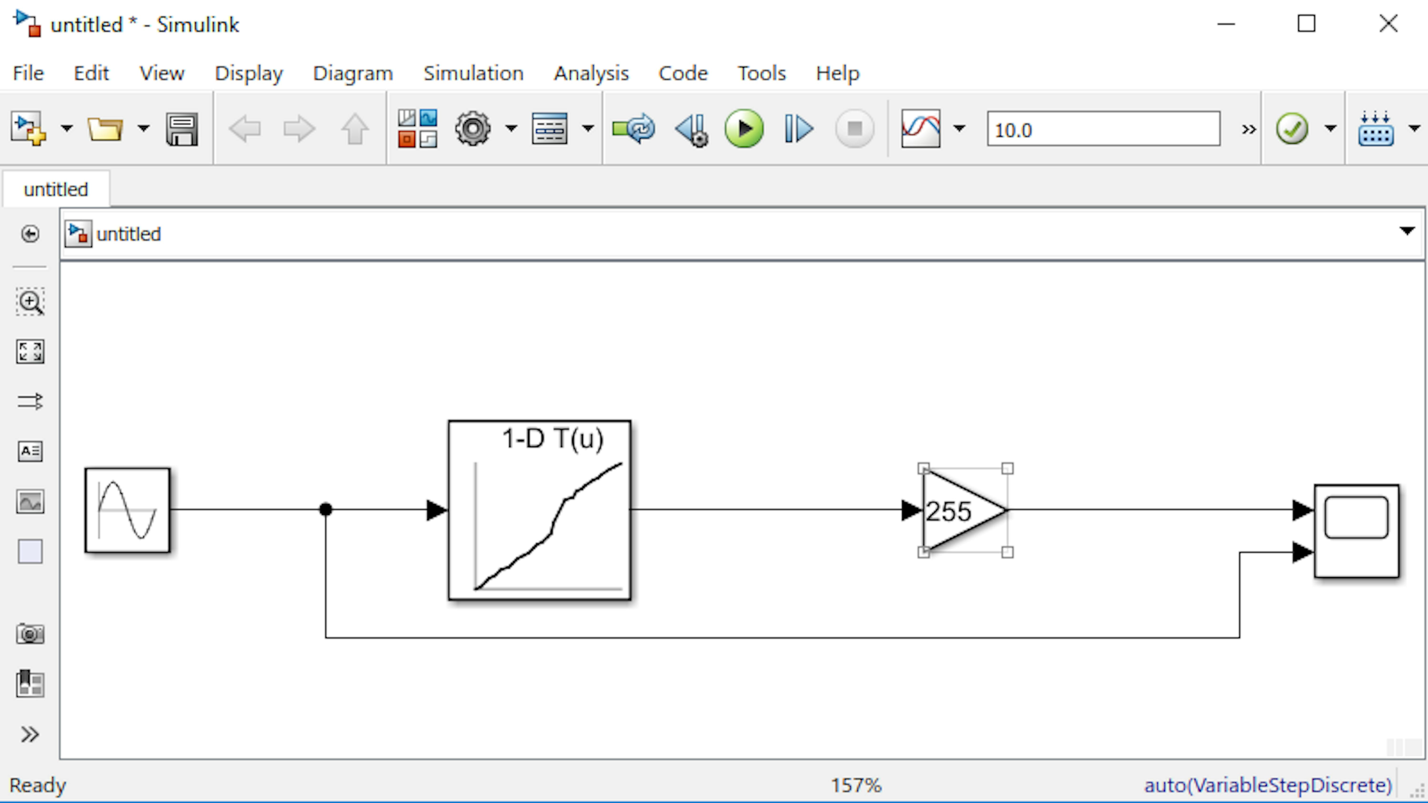
Rerun the model and examine the relationship between PWM command and input speed:
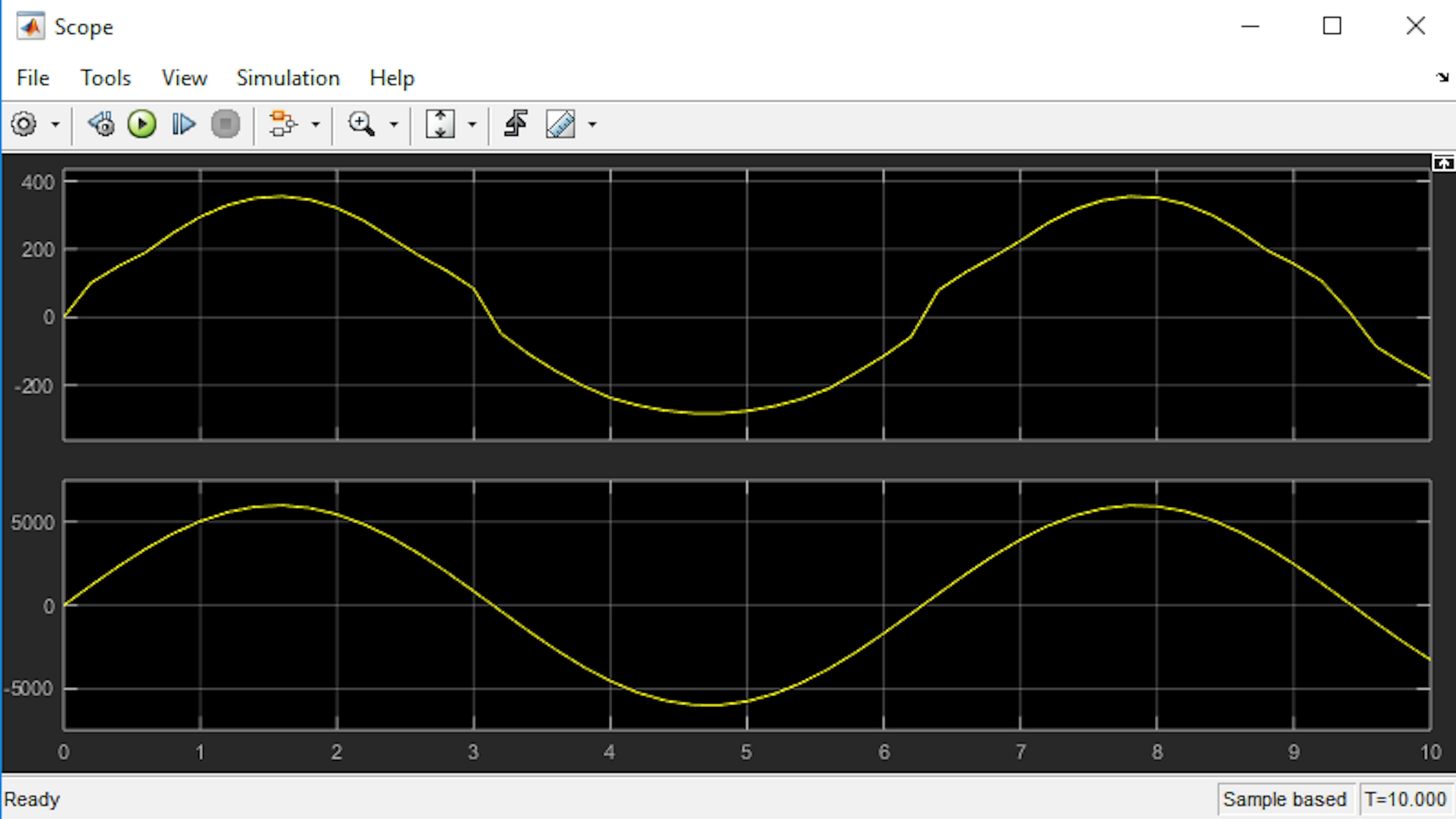
Just like you annotated your live script to communicate how your program works, you can similarly annotate a Simulink model to help explain it to others. First, let's label the blocks. By default, blocks do not display a block name. Click the Sine Wave block and change its label to speedInput:
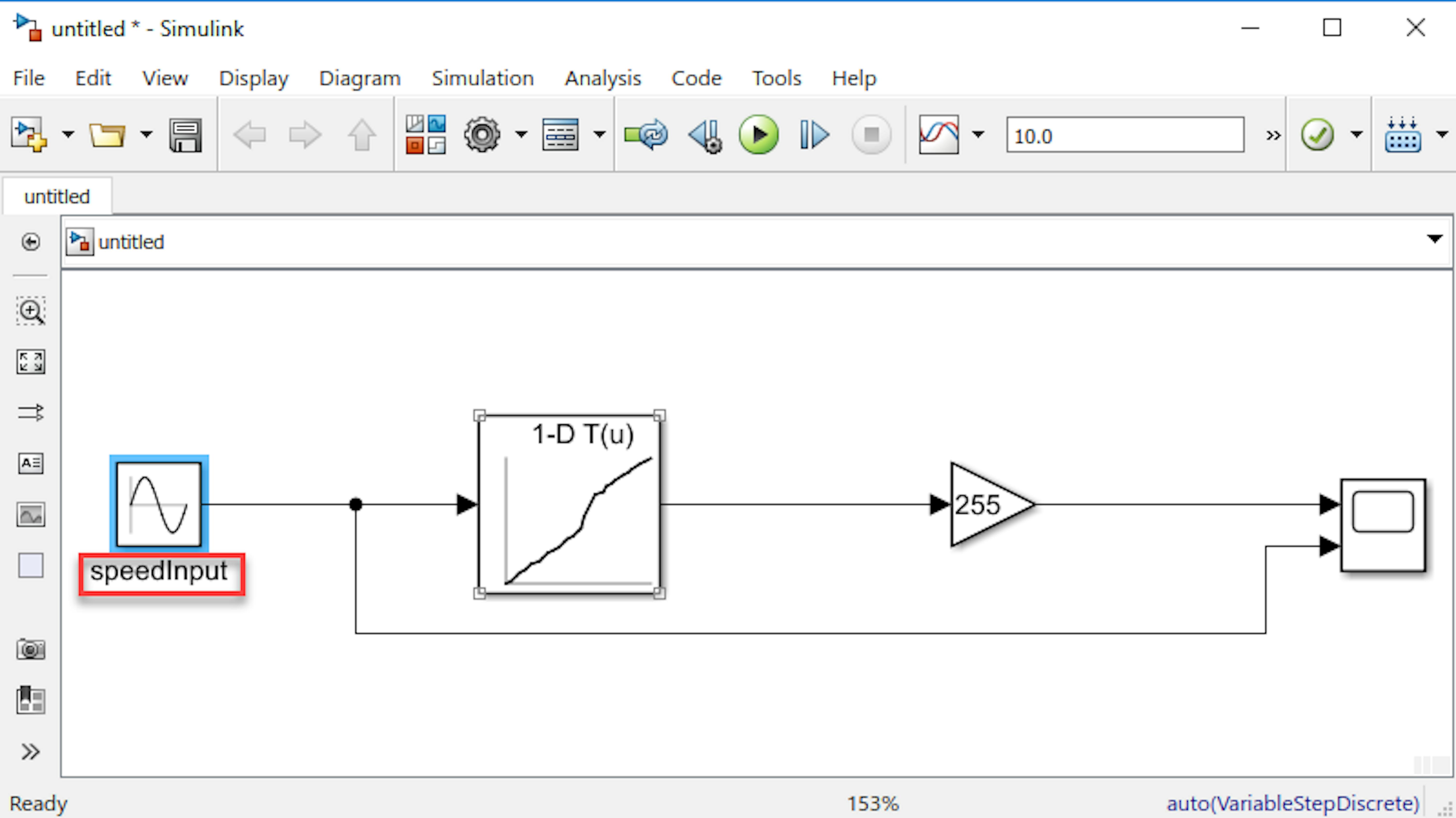
Similarly, label the next two blocks as shown in the following image:
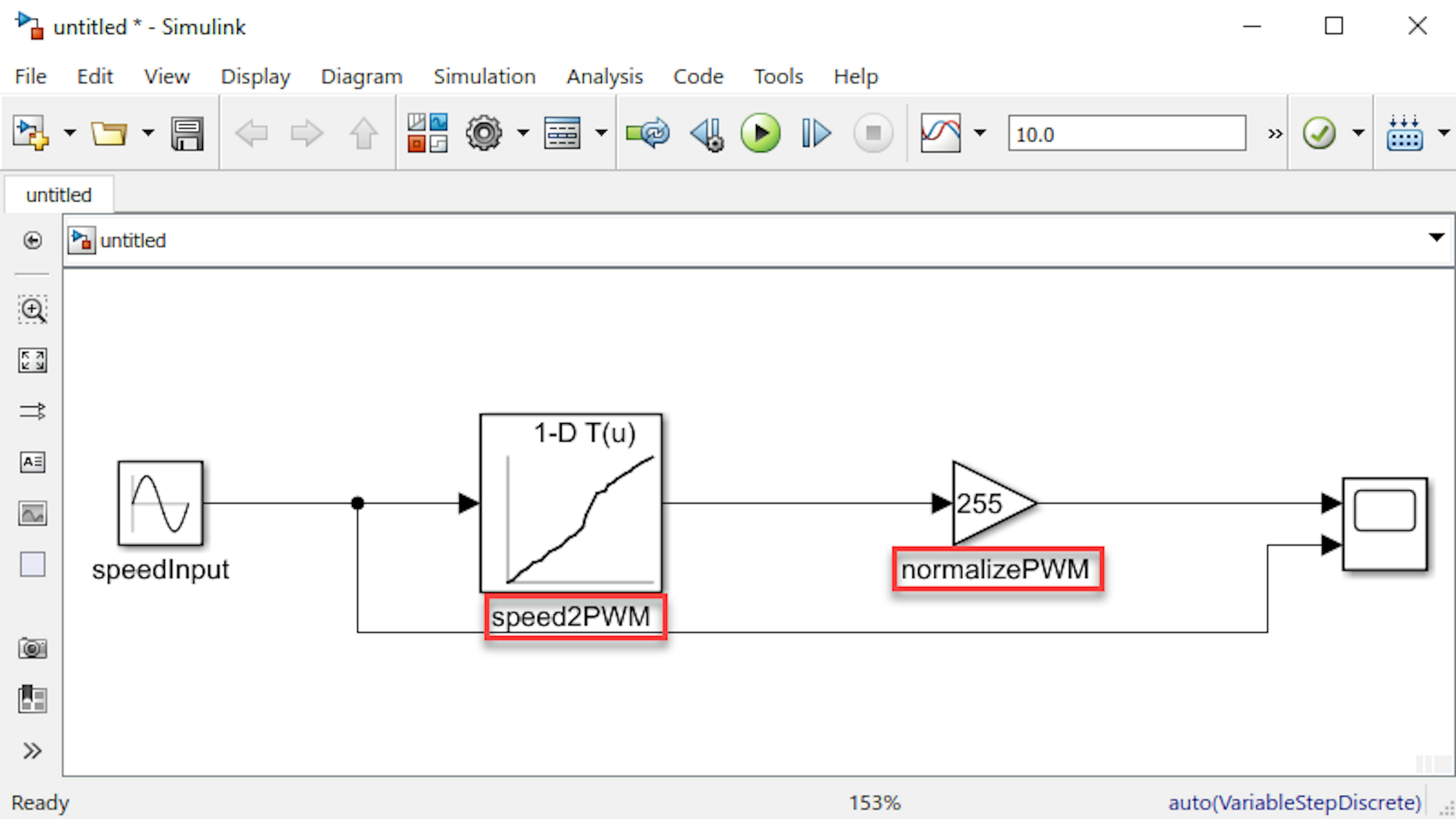
You can also label signals to indicate what quantity they represent. Double-click each signal line and add the following labels:
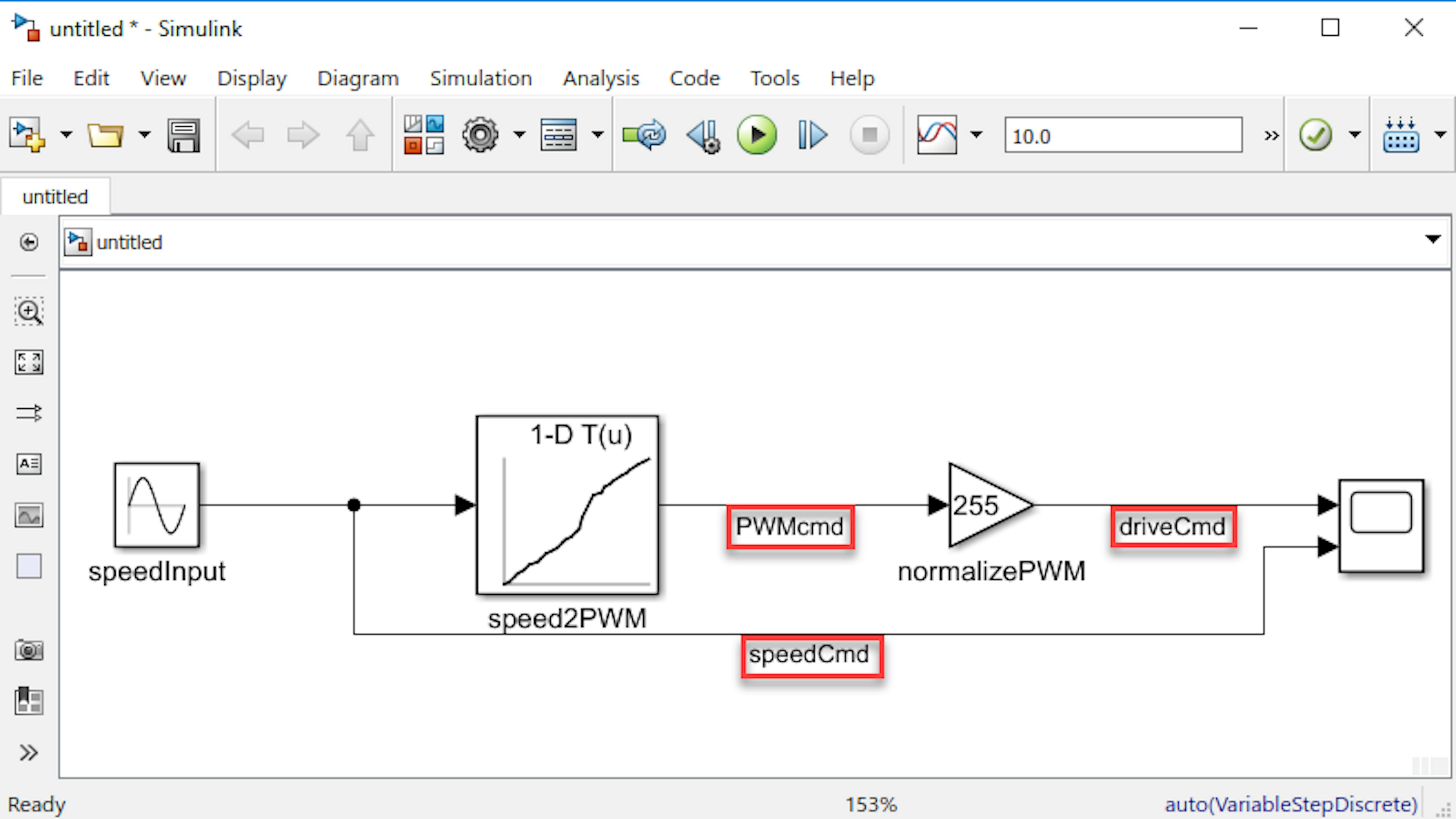
Note: You can click and drag signal labels to different locations along the signal line. Run the simulation again. Notice that your signal labels now show as titles in the Scope window:
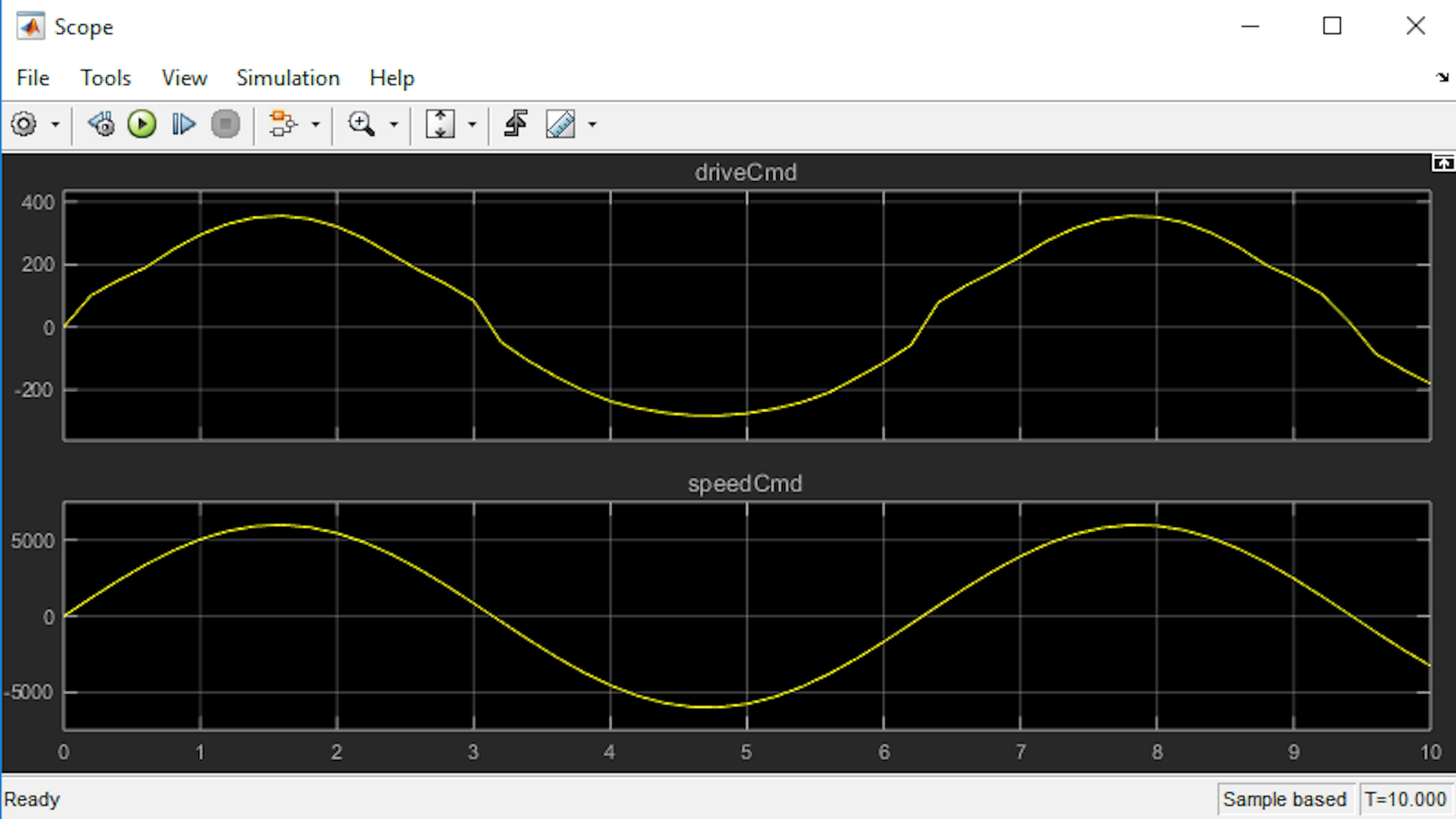
Right now, the simulation is running in continuous time. That means that all signals are treated as continuously varying values, and visualizations such as the Scope block show signals as smooth curves (although they are actually a series of discrete points connected by straight lines). Soon you will upload and run this algorithm on the Arduino board, which executes in discrete time. That means signal values are calculated and updated at periodic intervals. Let's adjust the model to simulate in discrete time so that we understand how it will work on the MKR1000 board later. In the Sine Wave block parameter dialog, set Sample time to Ts and click OK:
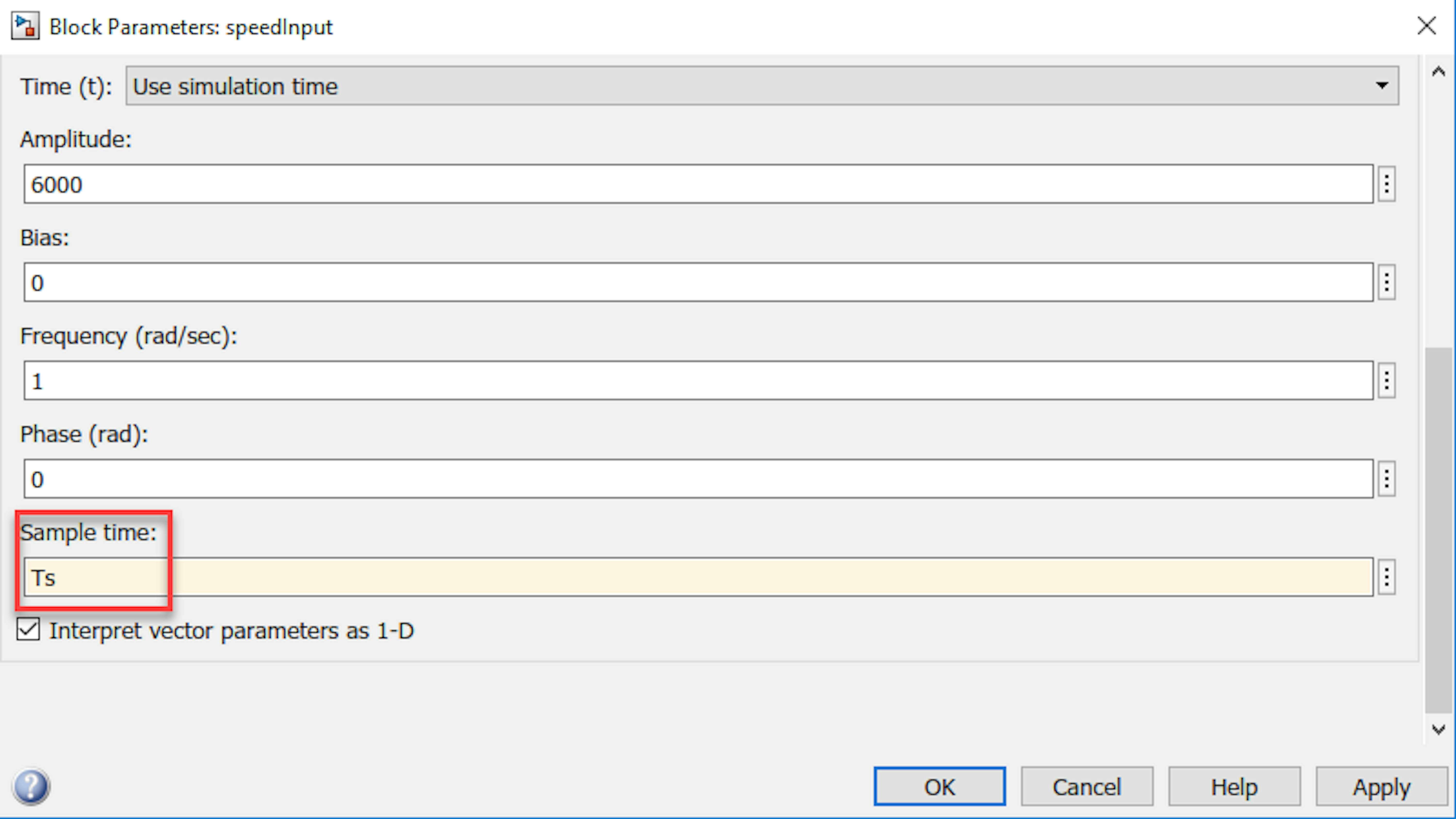
Now define Ts in the Command Window:
>> Ts = 0.1;
Run the simulation, and examine the scope:
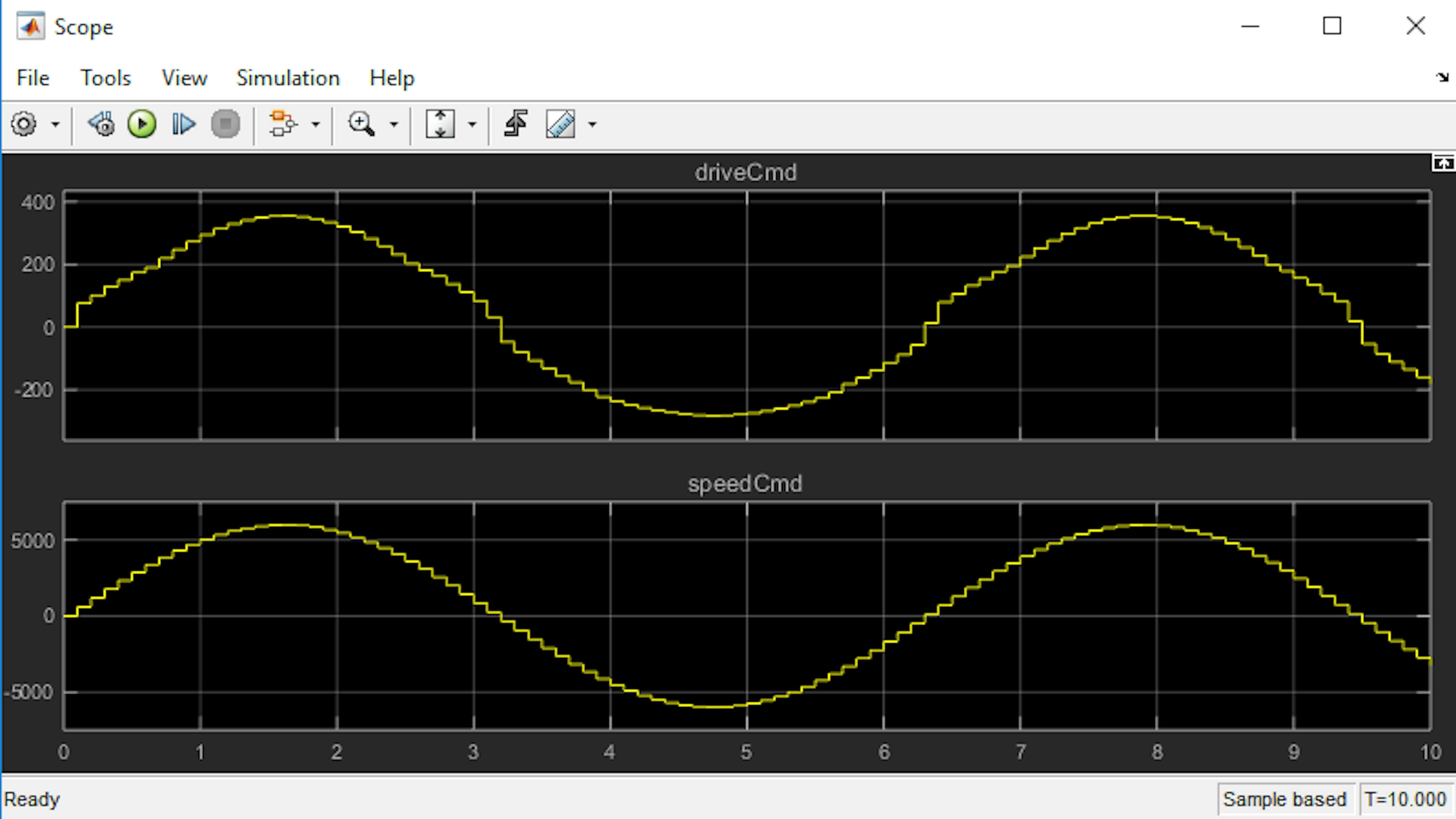
Note that the signals now display as flat values that hold for the entire sample time of 0.1 second. When modeling with discrete sample times in Simulink, it is helpful to color-code the model by sample rate. To do this, click Display > Sample Time > Colors:

Press Ctrl+J in the model window to view a legend of sample time colors. Note that this model has only one discrete rate, and it is derived entirely from the Sine Wave block's Sample time property. In this subsection, you learned how to simulate a model in continuous and discrete times. This is needed to build an understanding of how the code you created for Simulink will run on an Arduino board later.
ORGANIZING A MODEL
To complete this lesson, let's organize the model. You can compartmentalize a block diagram into smaller units, called subsystems. This is important to do when the complexity of your model increases, so that it is easier to read. The blocks we have added thus far comprise the motor controller. Later we will add more complexity to the controller, but for now, we can package it into a single subsystem block. Click the left mouse button and drag a box around the Lookup Table block and the Gain block:
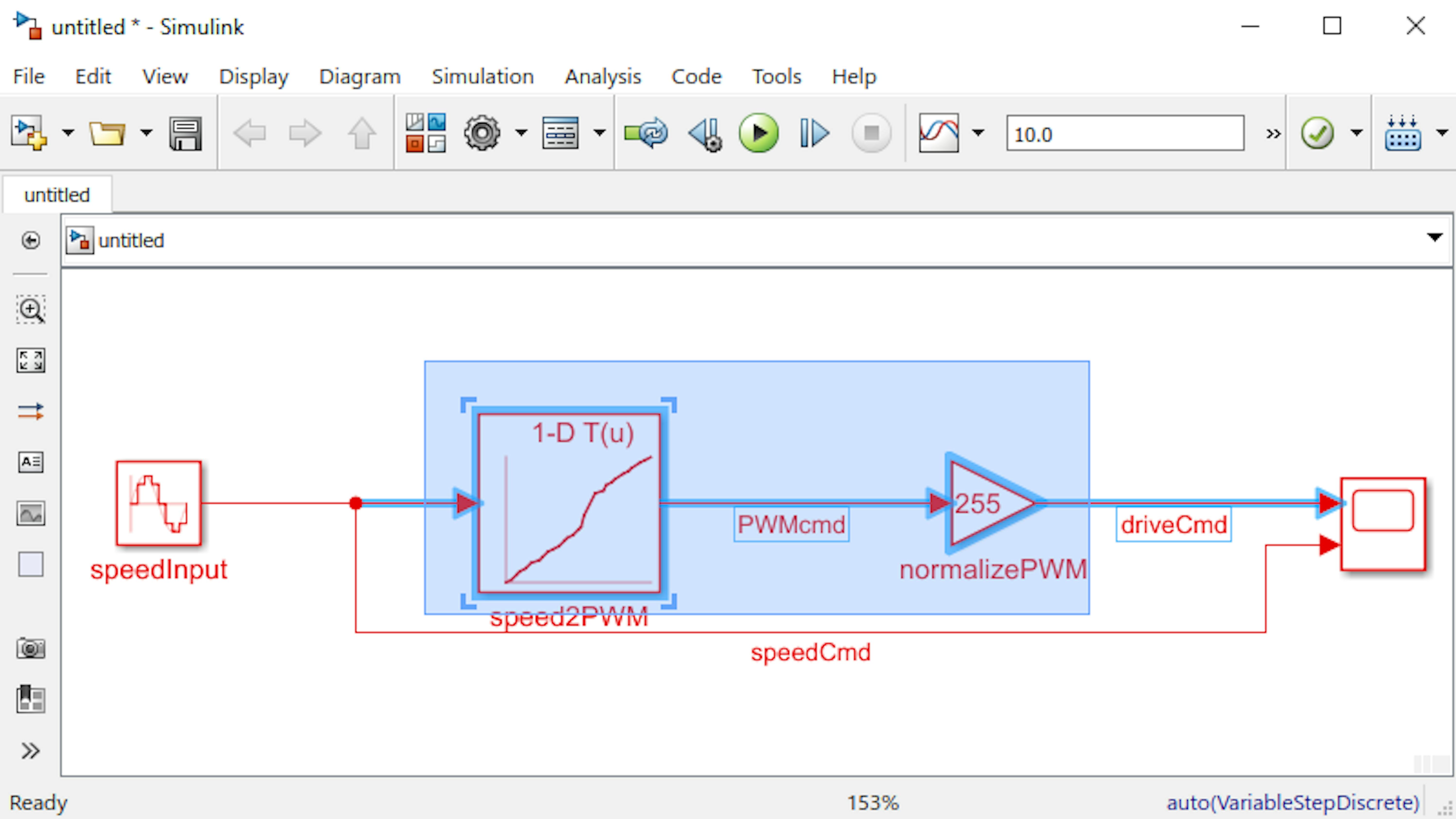
Now right-click either of the selected blocks and select Create Subsystem from Selection. Resize the block so that the port labels are visible:
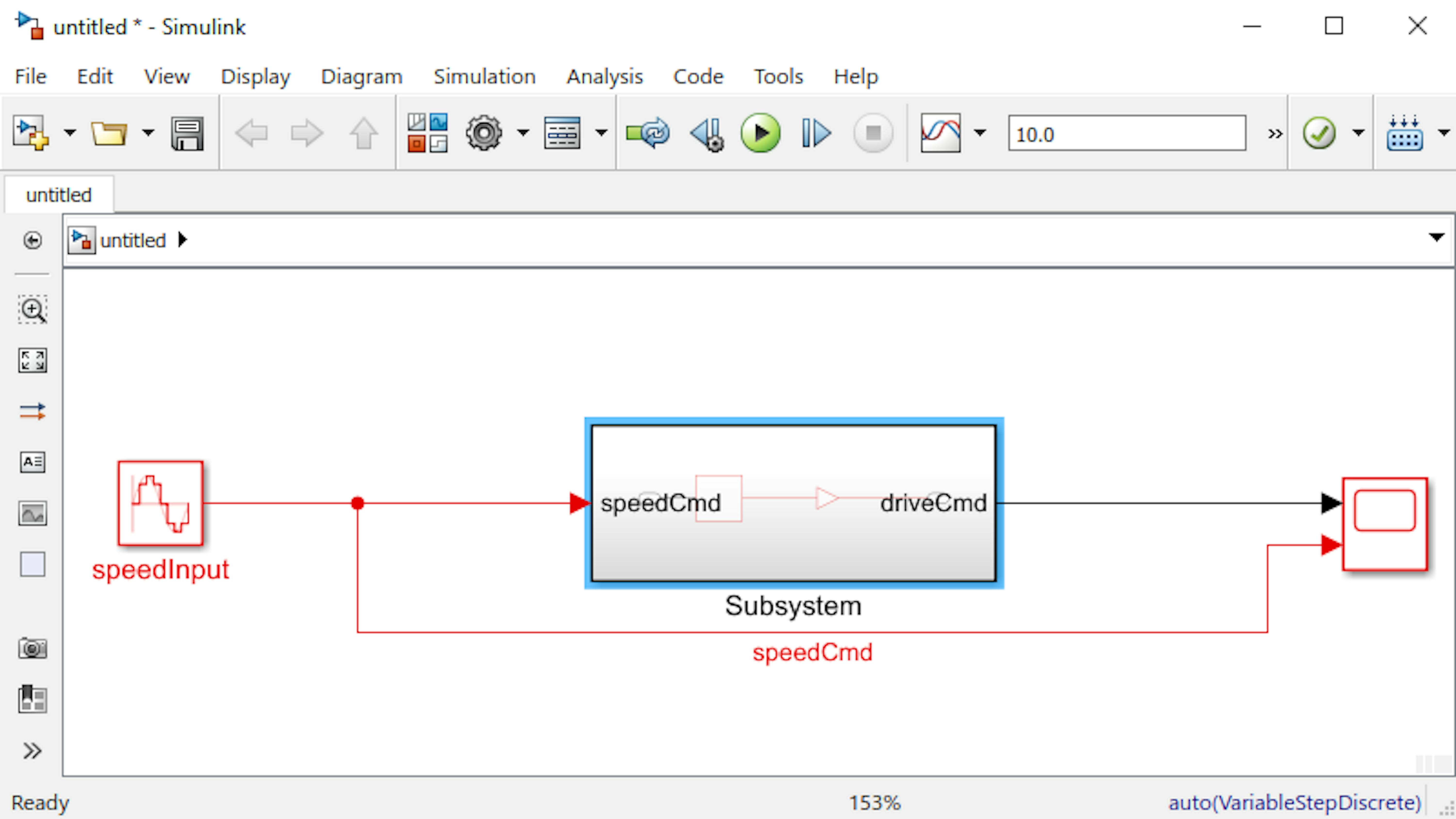
Finally, rename the subsystem block Controller:
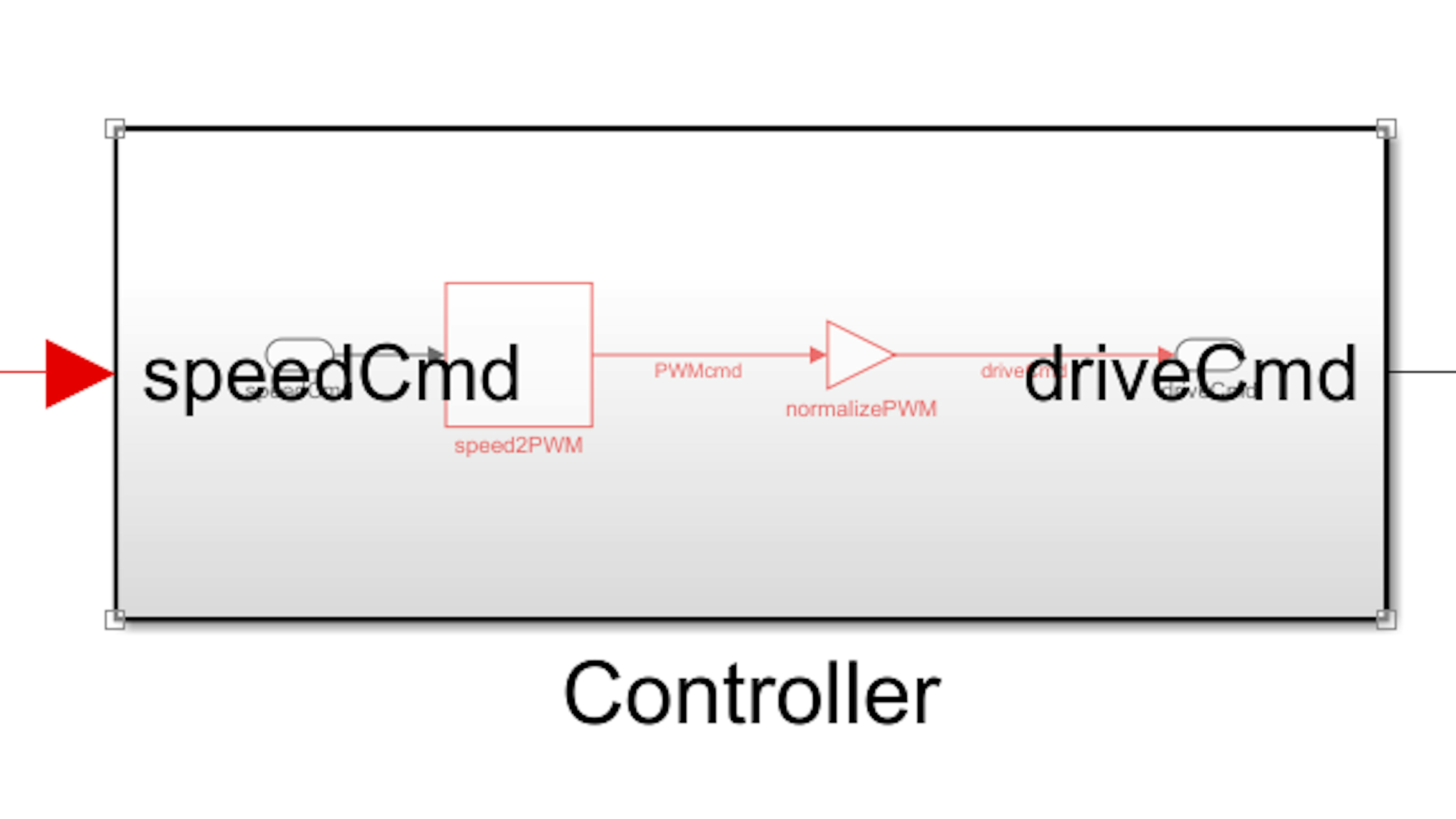
Notice that the port labels were derived from the original signal labels. Double-click the Controller block to view the contents inside:
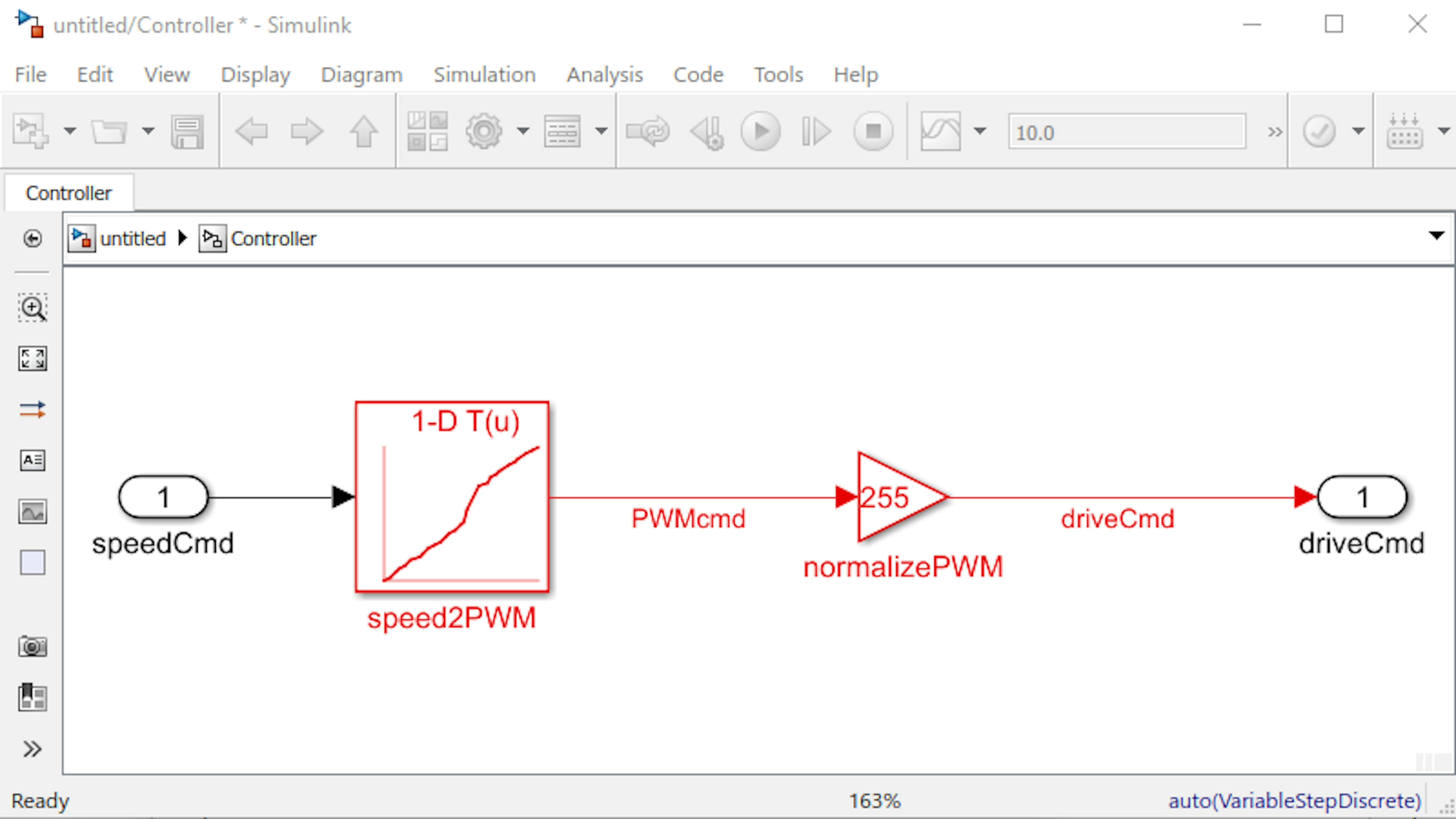
Now click the model name in the upper-left corner to get back to the top level of the model:
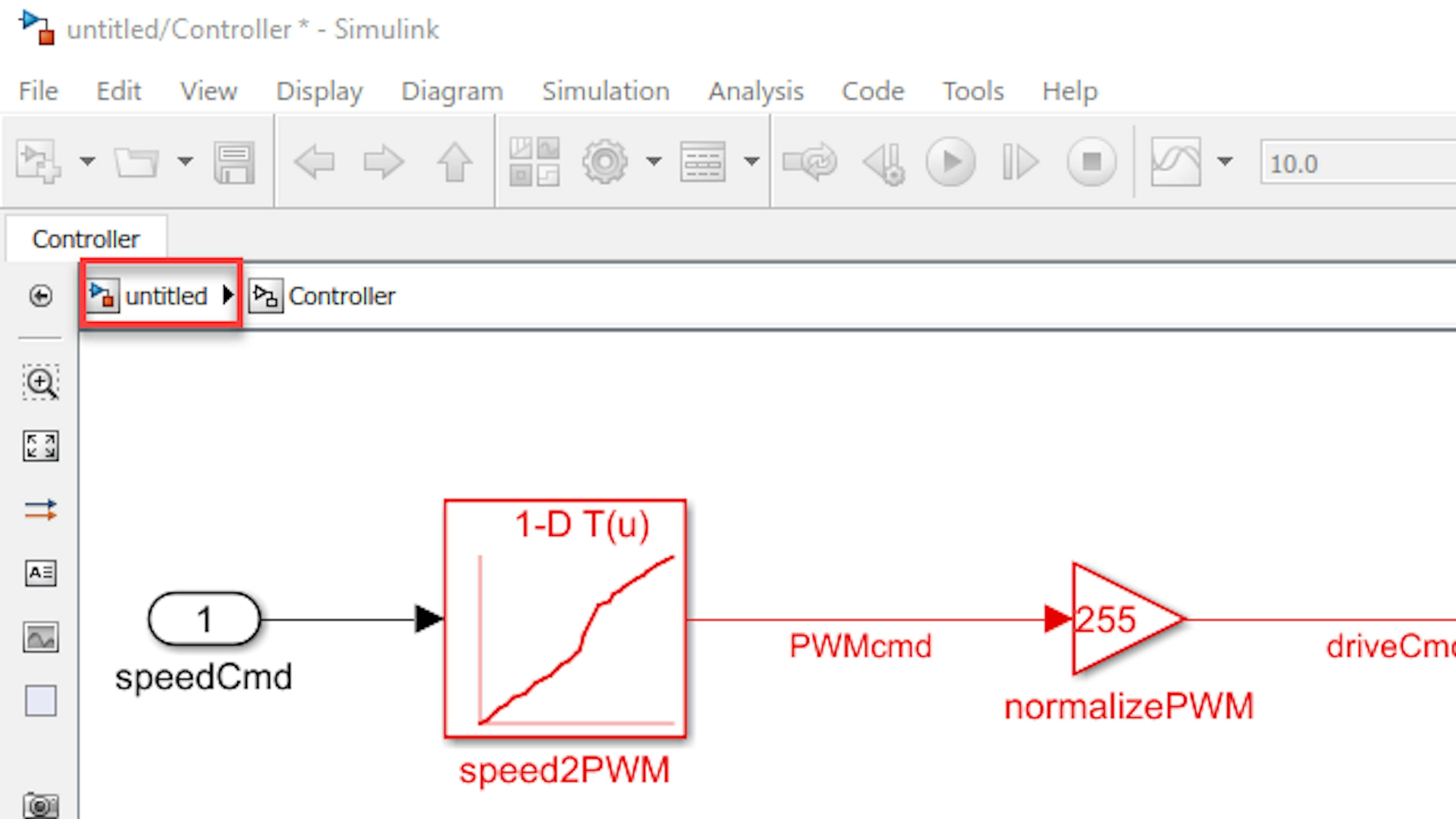
Run the model and view the scope to confirm it still behaves the same way as before.
Now save your model as myDCMotorControl.slx.
RUNNING SIMULINK MODELS ON ARDUINO
While you can write C code to upload it to Arduino boards, Simulink offers a great interface to program boards directly from its UI using blocks. The Simulink blocks can translate into code that can be compiled and uploaded to the board. This feature, which we introduce here, will be used later in the projects. In this section, you will learn:
- How to implement external sensors and actuators in a Simulink model.
- How to model basic mathematical and discrete dynamics in Simulink.
- How to condition signals in a Simulink model to be compatible with external device input and output formats.
- How to build and run a working Arduino application from a Simulink model.
- How to adjust model parameters while the application is running on Arduino and interpret the results.
- About the difference between open-loop and closed-loop control.
- How to run an Arduino application as a standalone program, outside Simulink.
In this lesson, you will add device driver blocks to your Simulink model to communicate with the DC 100:1 gearhead motor and the magnetic encoder. You will run your application directly on the MKR1000 hardware while communicating with the board through your Simulink model.
In this section, you will explore open and closed loop control mechanisms for motors. If you want a brief introduction to those, scroll down to Section "Reading Encoder Count and Motor Speed", where we will introduce the concepts. You can also take a look at them in the different projects, where these controllers are implemented in more specific scenarios.
ARDUINO DEVICE DRIVER BLOCKS
Start by opening your motor control model from the previous lesson (if it is not already open) and loading your analysis data:
>> myDCMotorControl
>> load motorResponse
>> Ts = 0.1;
Note: You can alternatively open the provided model, DCspeed2PWMsubs.slx, if you jumped over to this step and skipped the previous sections in the chapter.
Now let's have a look at the Arduino Device Driver blocks. In the Simulink Library Browser, navigate to Simulink Support for Arduino MKR Motor Carrier, and examine the blocks inside:
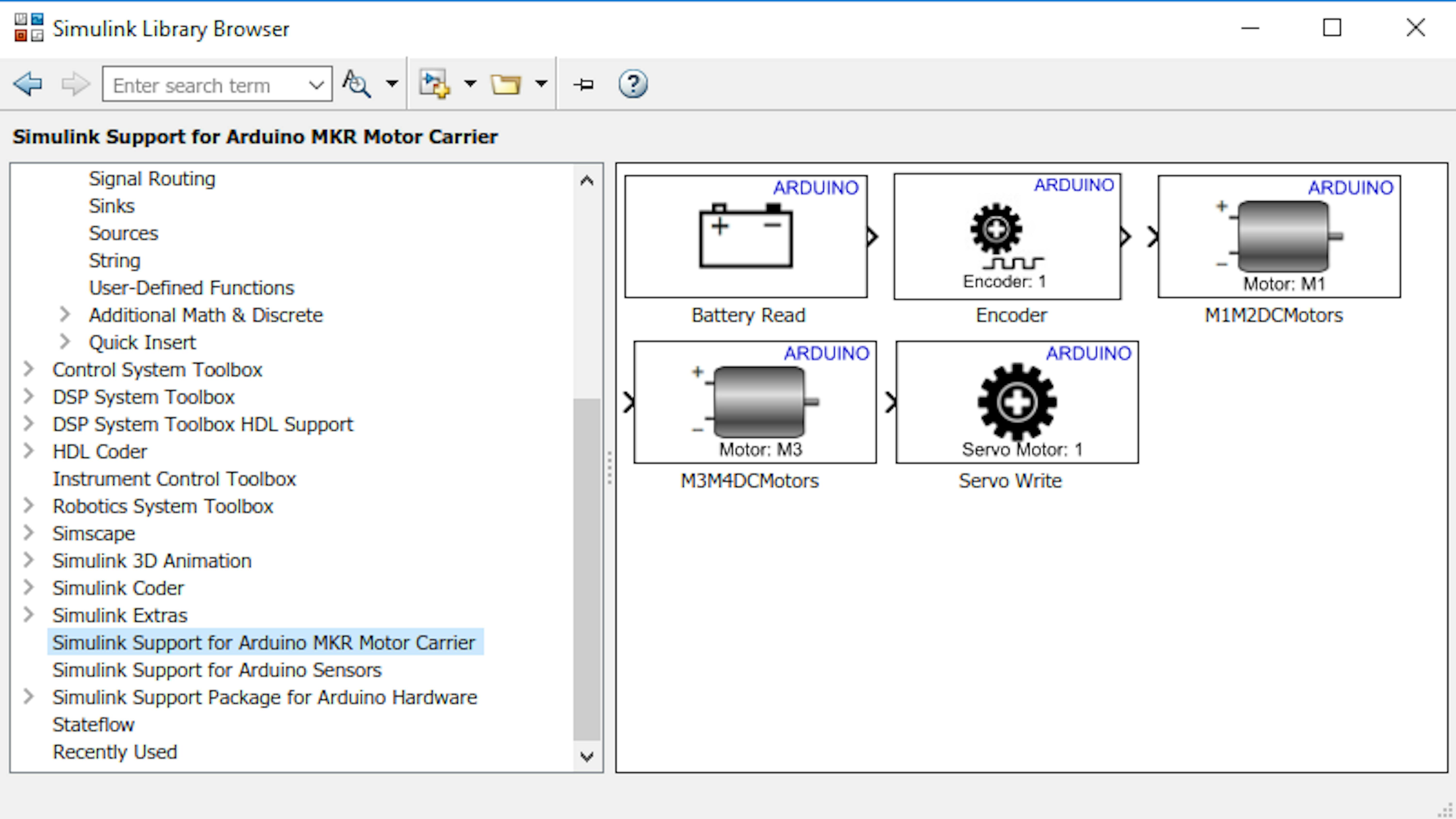
Notice that all the blocks are either source or sink blocks. This is because they represent the boundary between the Arduino processor application (which you are modeling in Simulink) and external devices, like the DC motor and magnetic encoder.
DRIVING A DC MOTOR
Let's start by communicating with the DC motor. Locate the M3M4DCMotors block in the Simulink Support for Arduino MKR Motor Carrier library, and drag it into your model:
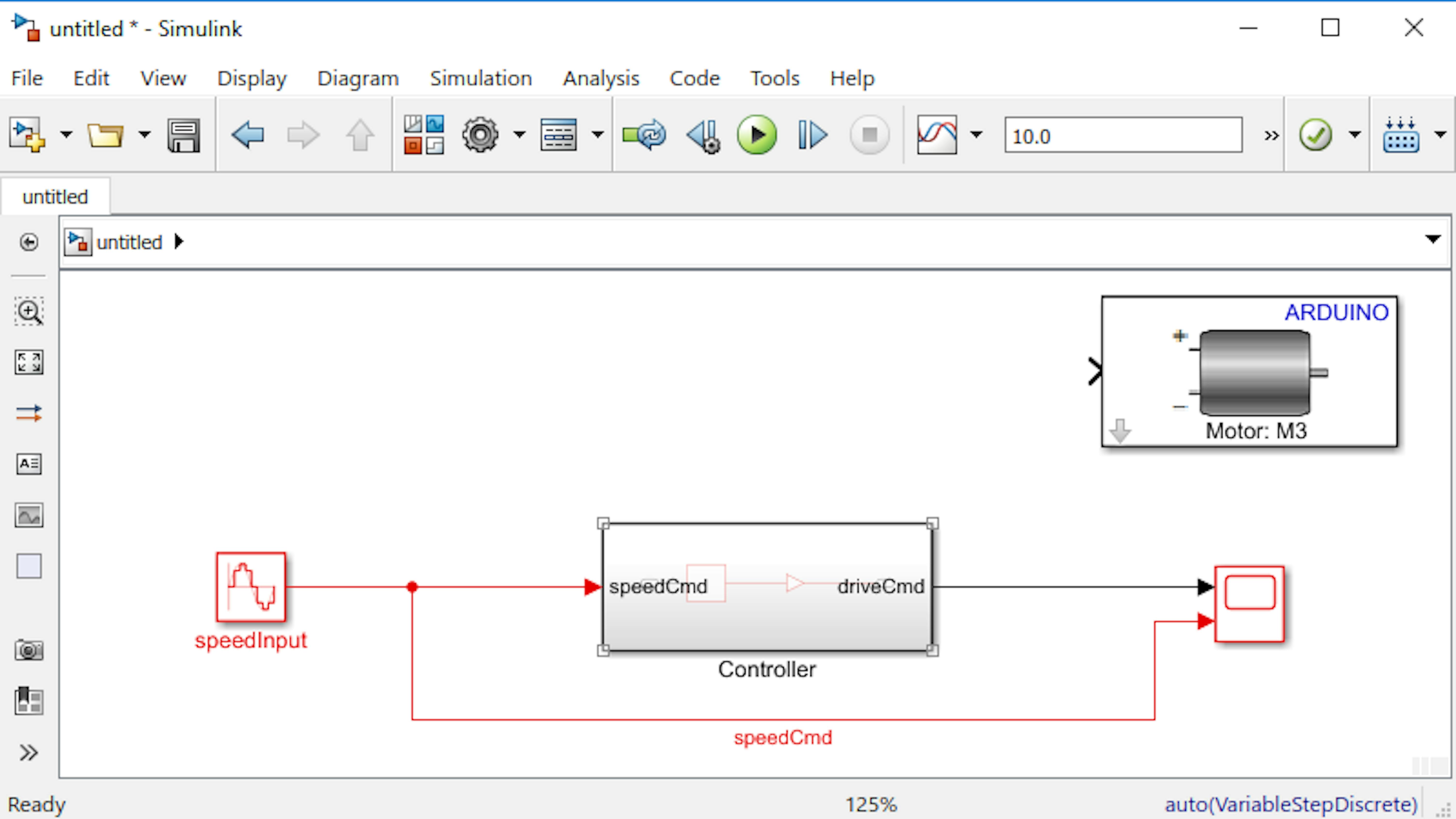
The M3M4DCMotors block requires one input signal, which is the drive command expressed as a value between -255 and 255. Double-click the M3M4DCMotors block, and configure it as shown in the image below:
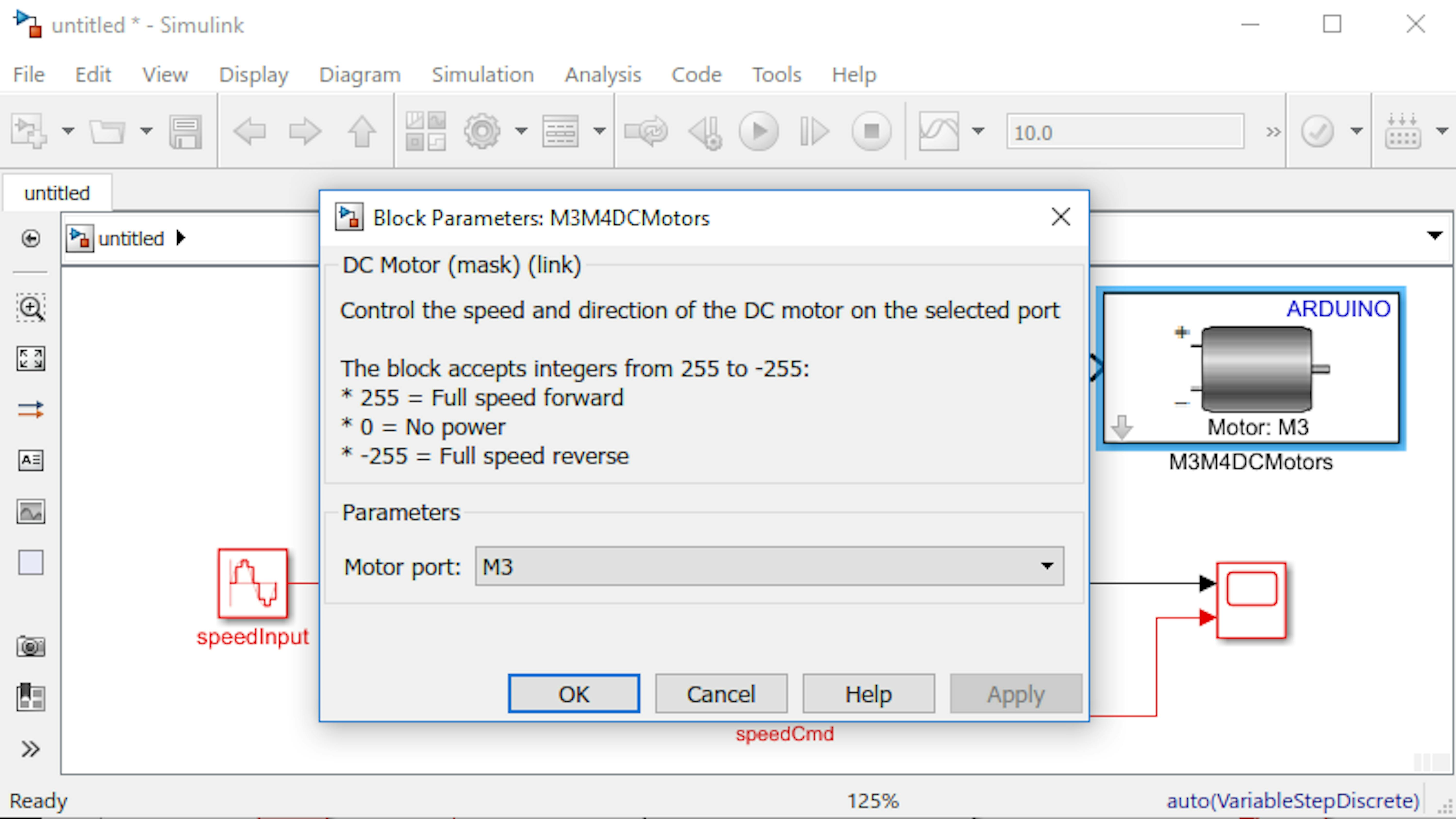
The Motor port property maps the block to one of two labeled DC motor ports (M3 or M4) on the Motor Carrier. Create a new branch of the driveCmd signal by right-clicking and dragging the mouse from the signal line, and route the signal into the M3M4DCMotors block:
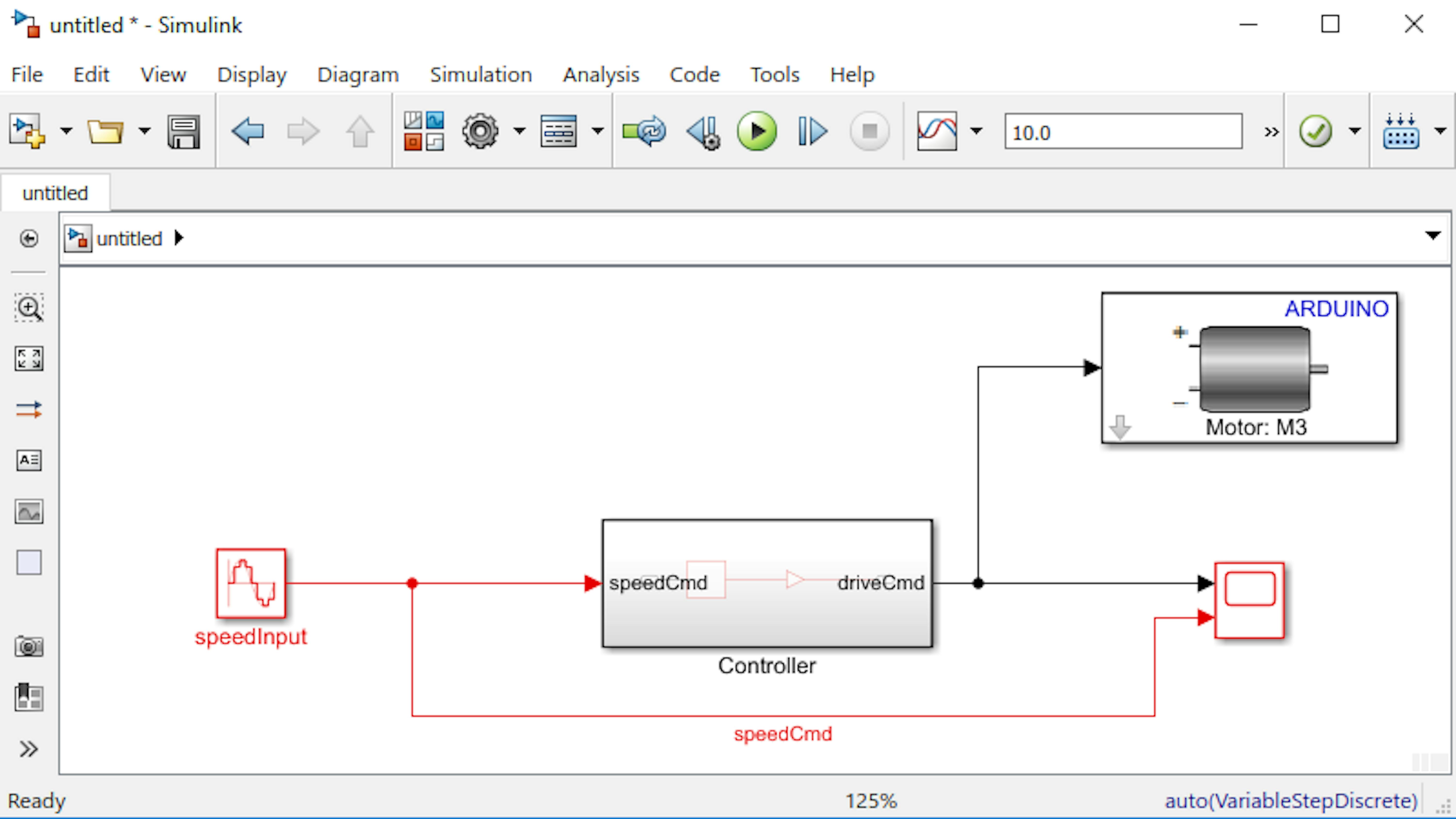
You're almost ready to run the software controller on the MKR1000 board! First, you need to configure the model to run on Arduino. Open the Configuration Parameters window by clicking the "gear" button:
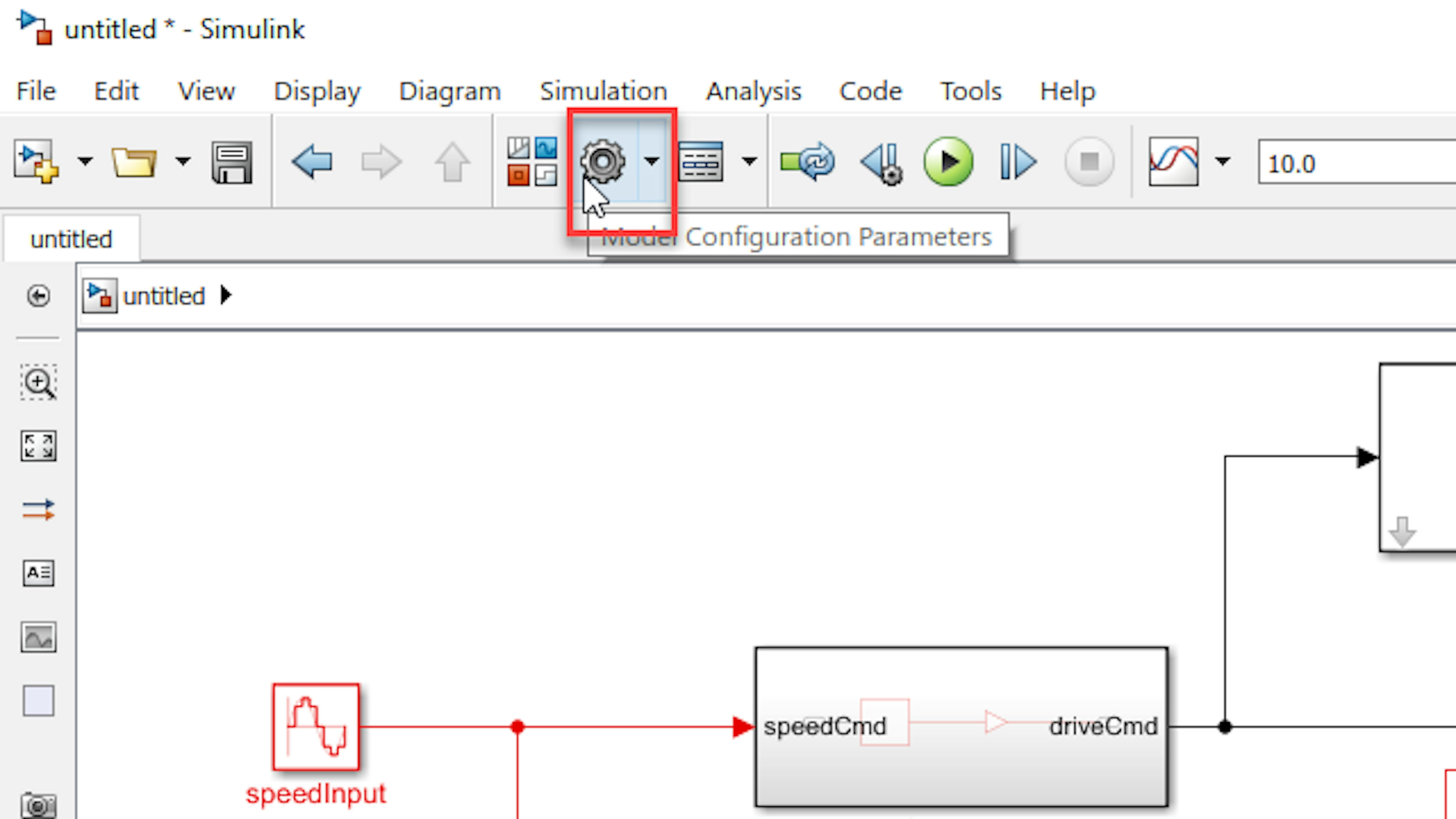
Configuration Parameters is a set of options where you configure how your simulation should run, what hardware you are running it on, and how the model algorithm should handle various run-time conditions. Navigate to the Hardware Implementation pane, and set Hardware Board to Arduino MKR1000:
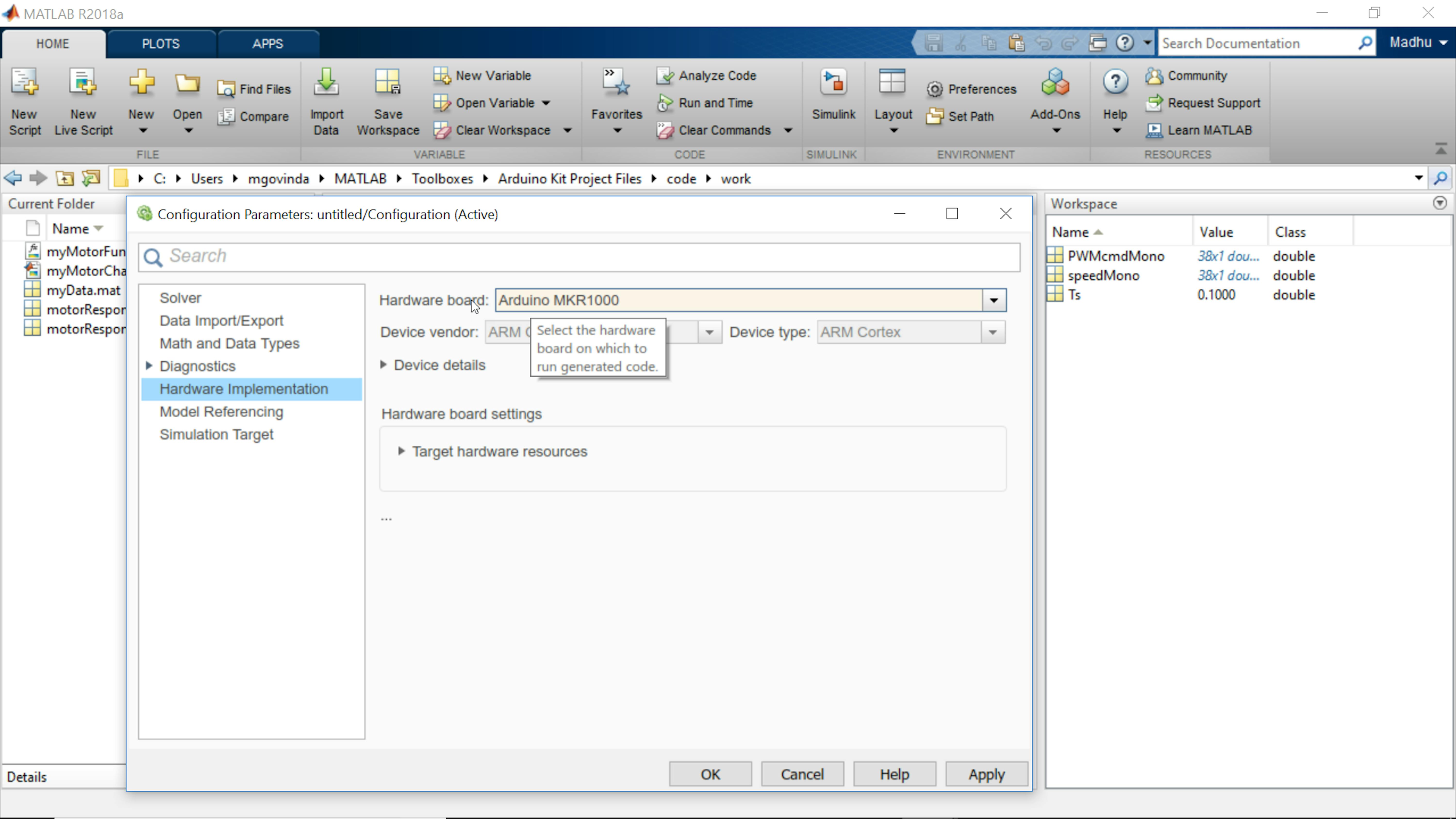
Note: Those who are on MATLAB Release R2019a or later, follow the next step to choose Serial as communication interface. In older releases this is the default option.
Go to Target hardware resources > External mode > Communication interface and choose Serial as shown below:
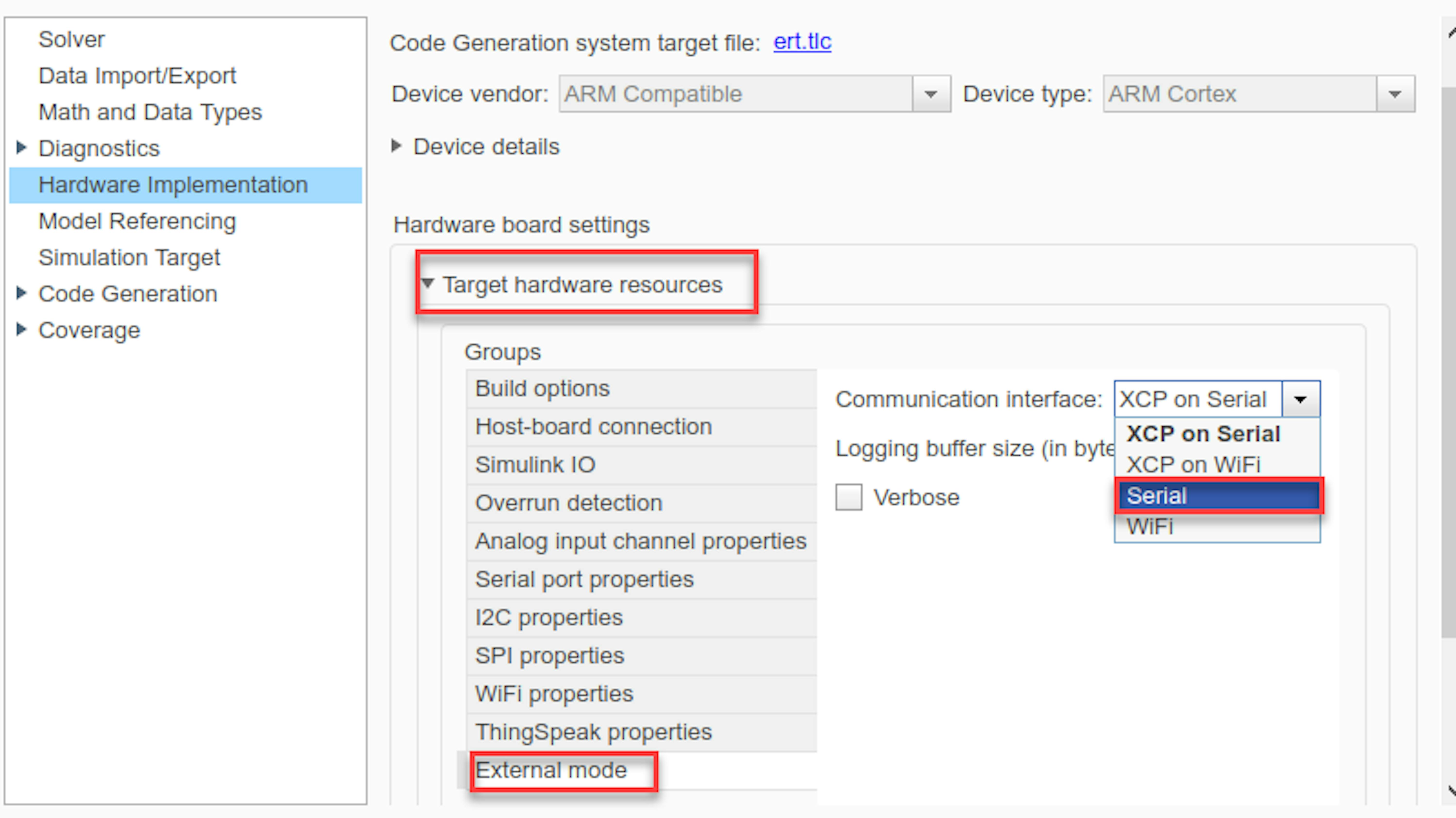
When you set the model to run on a specific board, some of the options throughout Configuration Parameters will set themselves automatically, as required. Click OK to return to the model window. Previously you have been simulating your model using normal mode. In normal mode, the default setting makes your model run on the computer without communicating with any external hardware. In normal mode, you can prove that your system works conceptually, before dealing with the details of implementing it on hardware.
To run the model on the MKR1000 board, you will use external mode. In external mode, Simulink builds an executable from your model and uploads it to the external hardware board. When the executable runs on the external hardware board, you can interact with the running application using the Simulink model. This enables you to monitor signals of interest and change parameter values in the model as it runs on the hardware.
In the model window, change the simulation stop time to Inf so that it will run indefinitely. Set the simulation mode to External, using the drop-down menu to the right of the stop time:
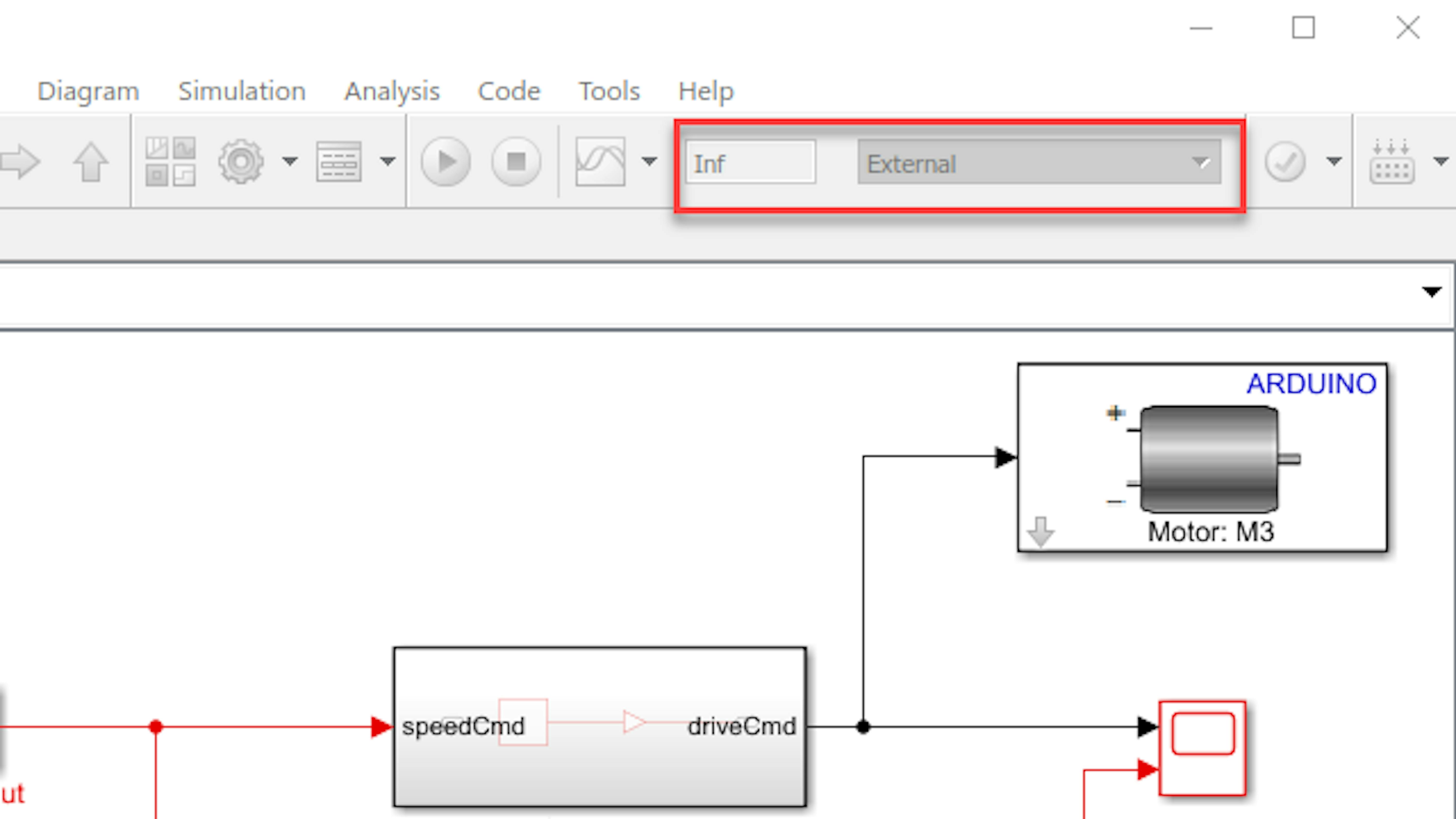
Turn on the battery power by using the ON-OFF switch on the Carrier board. Now click the Run button. You must wait for Simulink to build the executable and then initialize the external mode infrastructure.
Note: If the model gets stuck in the code generation mode for more than few minutes, a) try double pressing the reset button on your MKR1000 or b) it could be because you have an "arduino object" (like in "a = arduino;"). You won't be able to upload any Simulink model to the MKR1000 until you clear the "arduino object", because it is getting the COM port busy.
Once the application starts running, examine the oscillatory motion of the motor and magnetic encoder. Is the speed oscillating at the same rate as the input speed command? Stop the simulation, and then turn off the Motor Carrier power.
READING ENCODER COUNT AND MOTOR SPEED
You now have a functional control system that theoretically drives the motor at the desired speed. But how do you know it is working correctly? Let's set up the model to read the magnetic encoder count so that you can calculate the rotational speed and see how well it matches the commanded speed. Add an Encoder block from the Simulink Support for Arduino MKR Motor Carrier Simulink library:
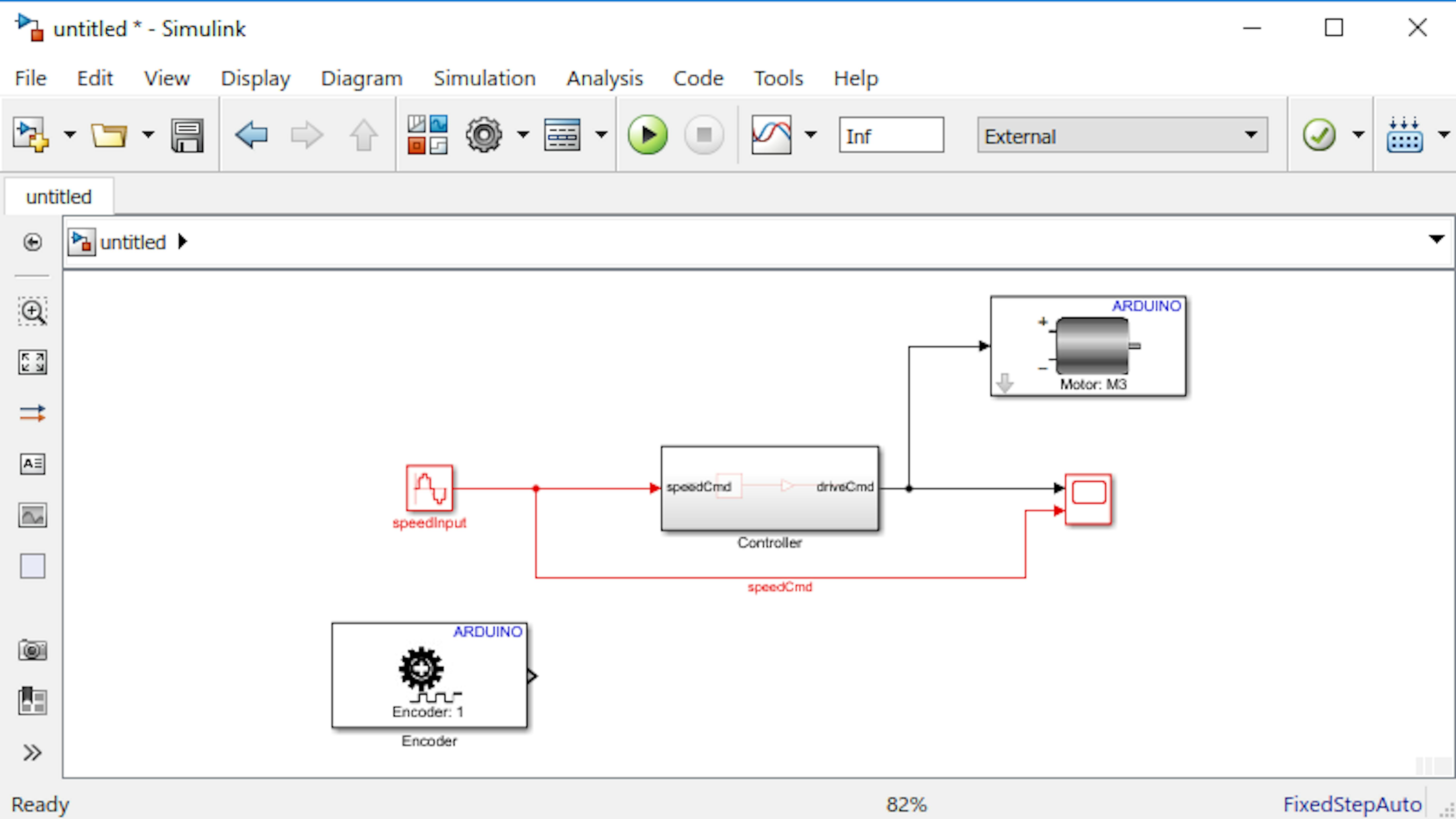
Open the block dialog and set the encoder number to 1 :
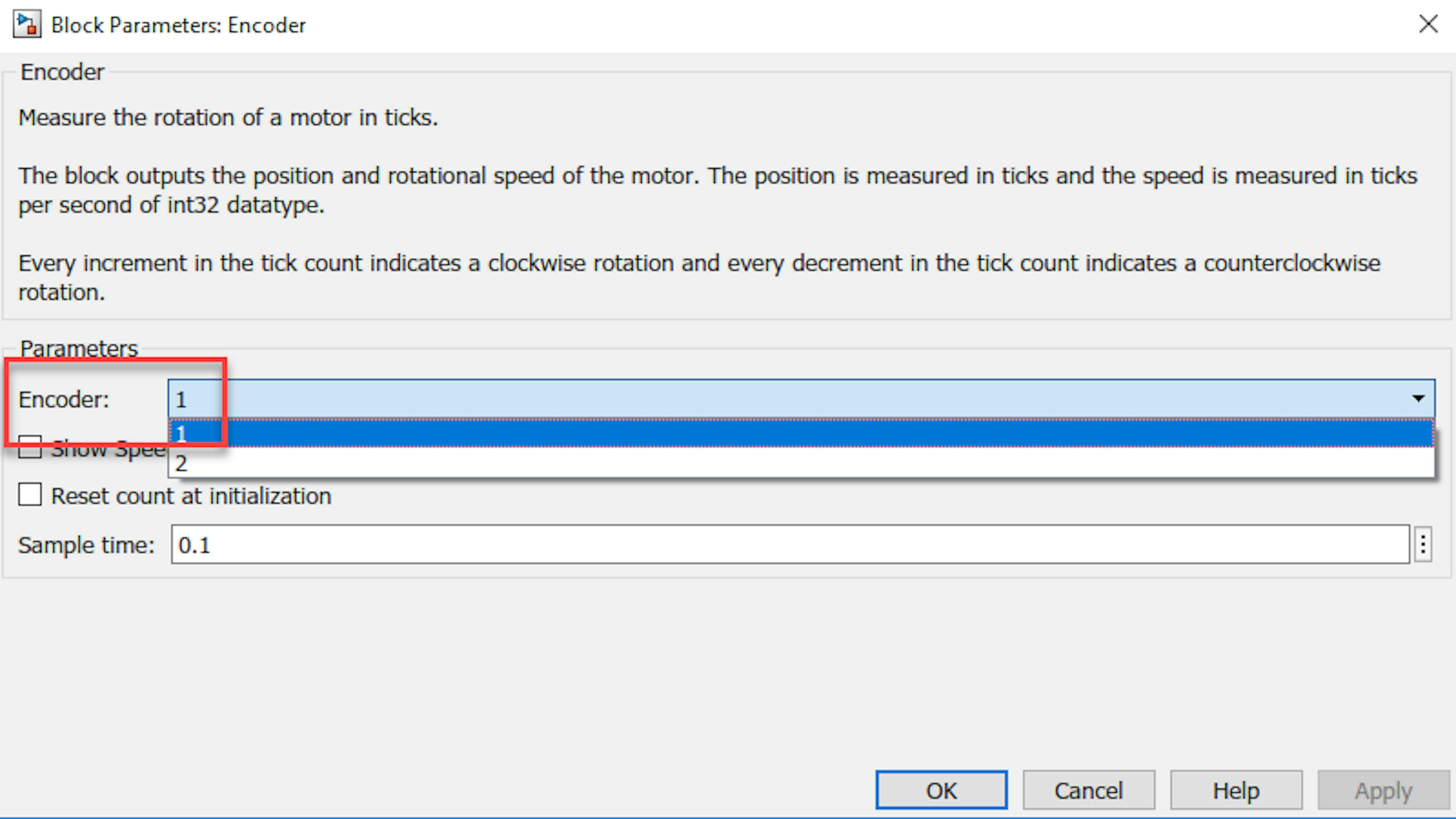
Let's test the Encoder block in isolation. Attach a temporary Scope block (from Simulink>Sinks) to the output.
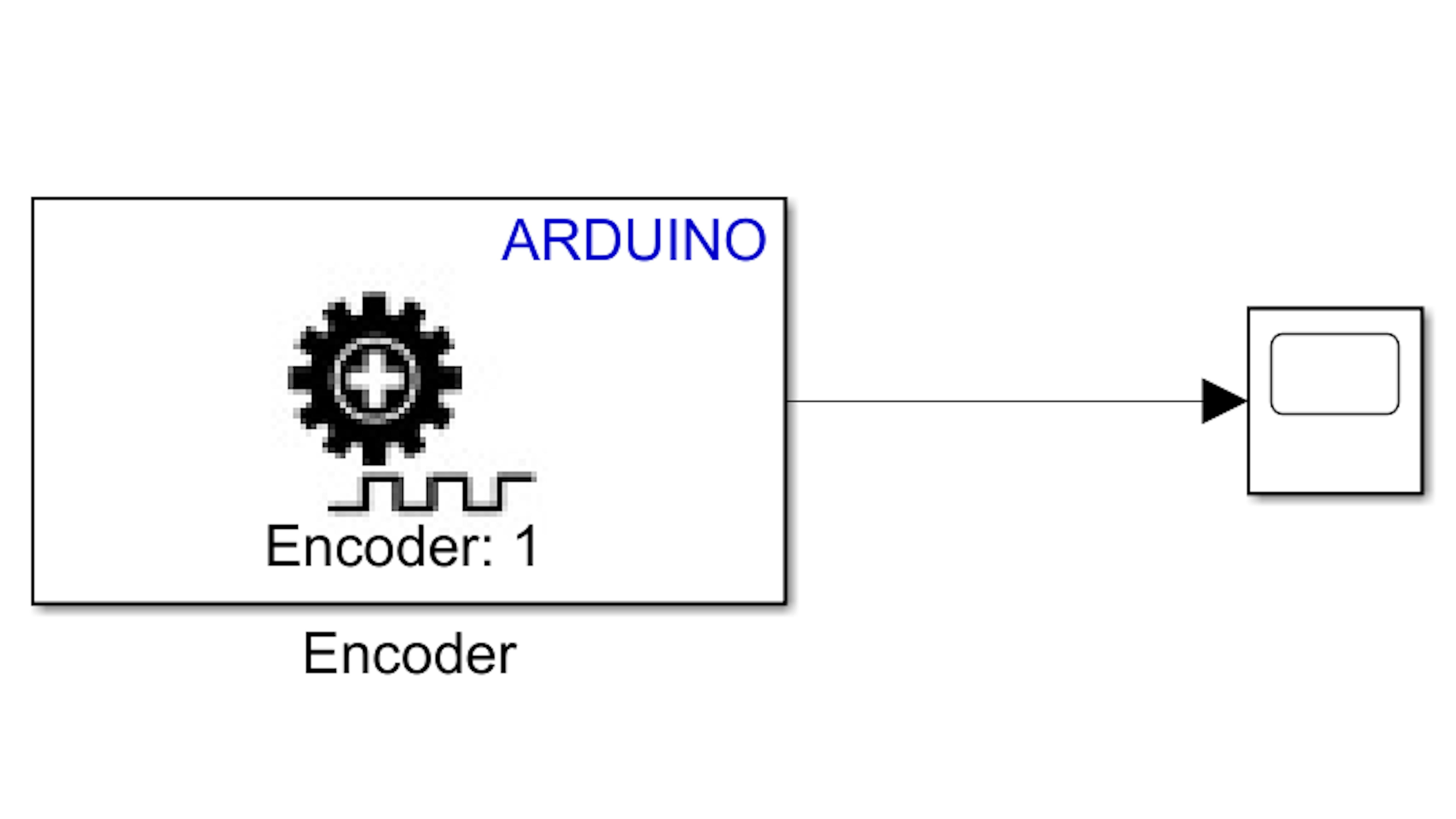
Now turn ON the Motor Carrier power switch and run the model. Watch the encoder count in the Scope block.
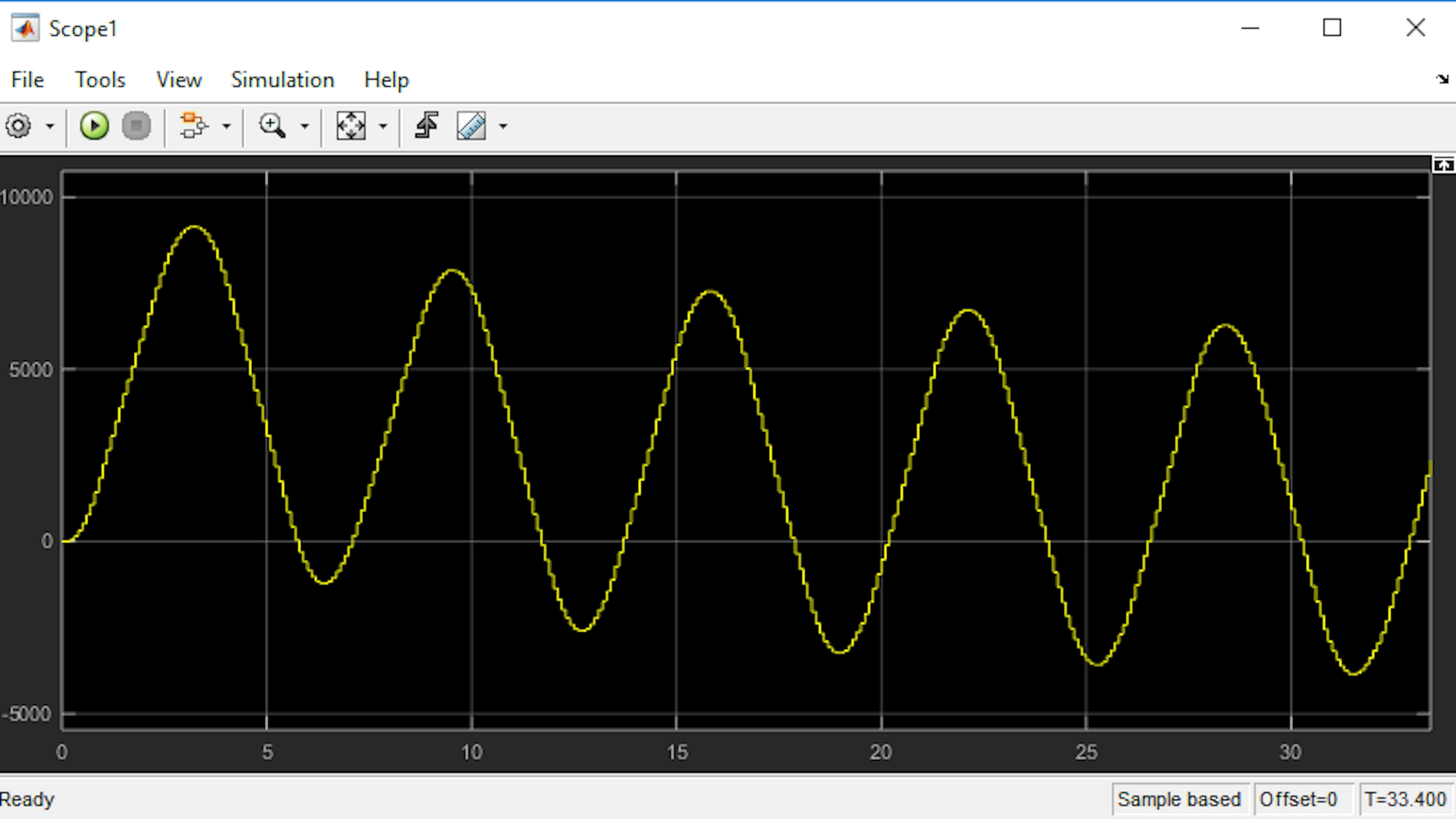
Note: You can zoom to the full vertical limits of your data by clicking the Scale Y-Axis Limits button in the Scope block:
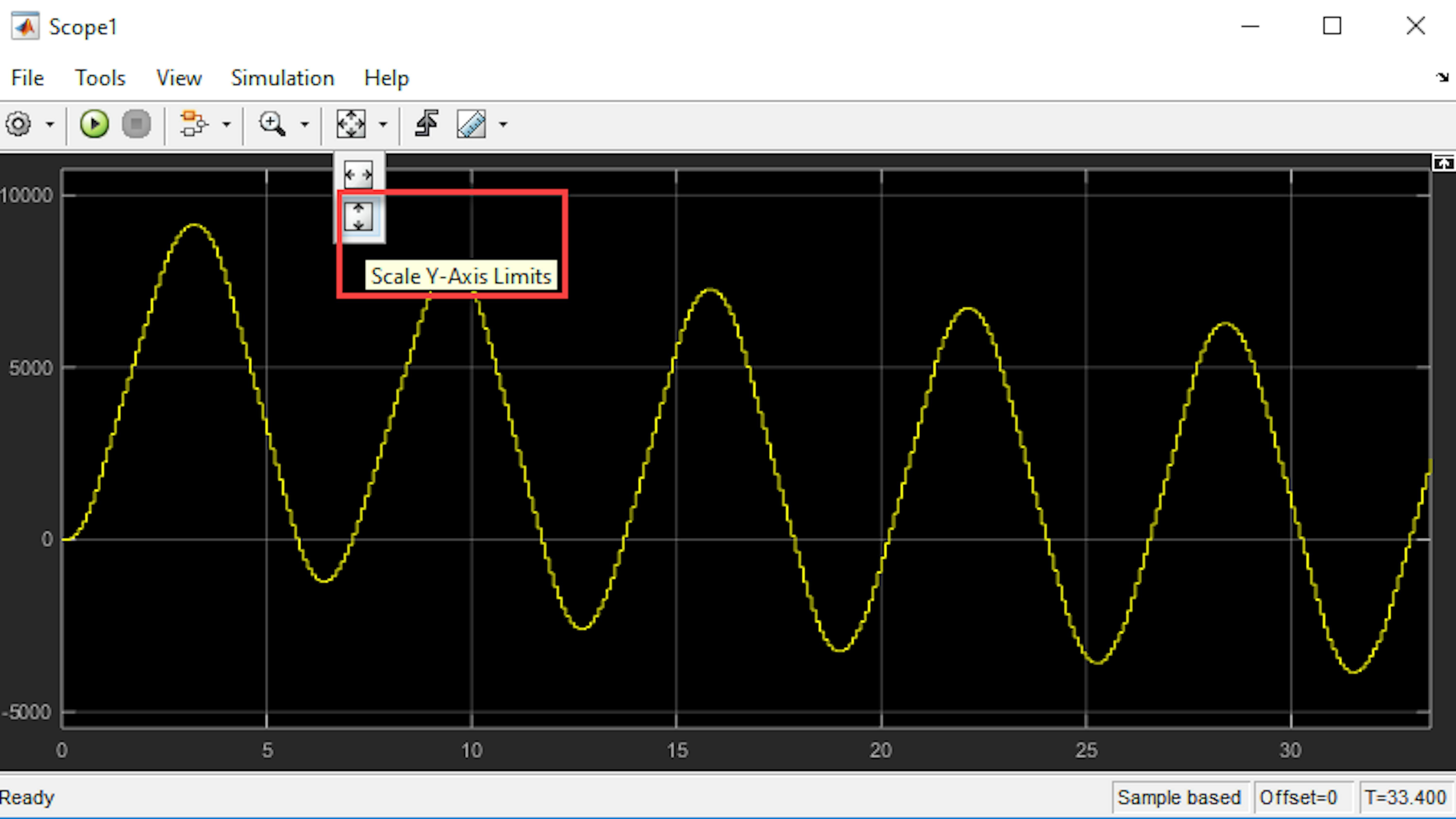
Next, let's calculate the angular speed. In the top level of the model insert three blocks: a Sum block (Simulink > Math Operations) with List of Signs '|+-', a Unit Delay block (Simulink > Discrete), and a Gain block with a Gain of 1/Ts.
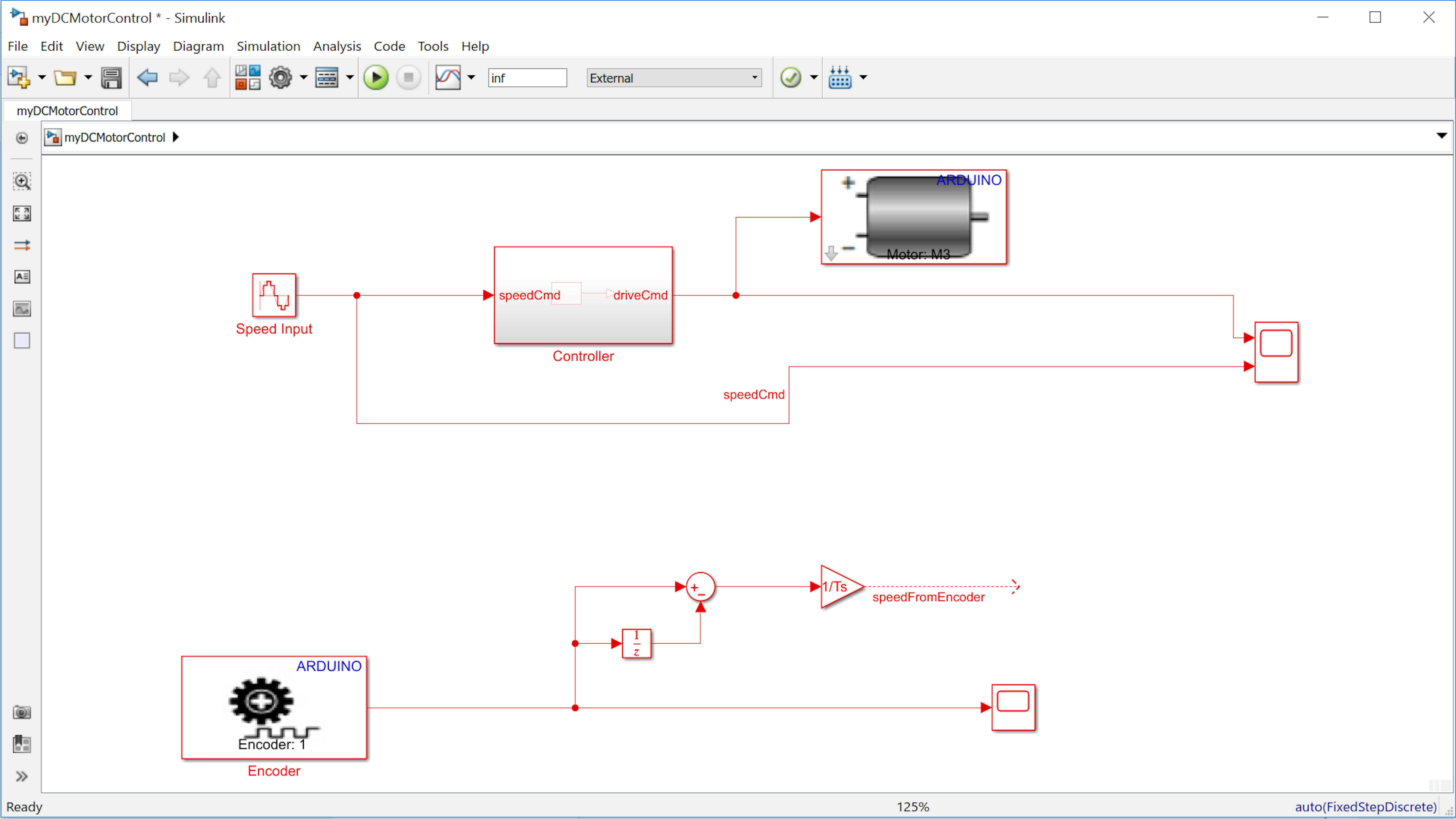
Note: There are two ways to change parameters such as List of Signs or Gain value that we saw above. 1) When you drag and drop the block the parameters show up by default and you can edit by typing there. 2) Double click on the block and enter the parameter value in the pop-up window.
Link the new blocks as shown above and name the output signal from Gain block as speedFromEncoder. This calculates the change in counts divided by the sample time, Ts. This is the equivalent to how we calculated the motor speed in previous chapter.
SPEED
Route the speedFromEncoder signal to the Scope block, creating a third inport:
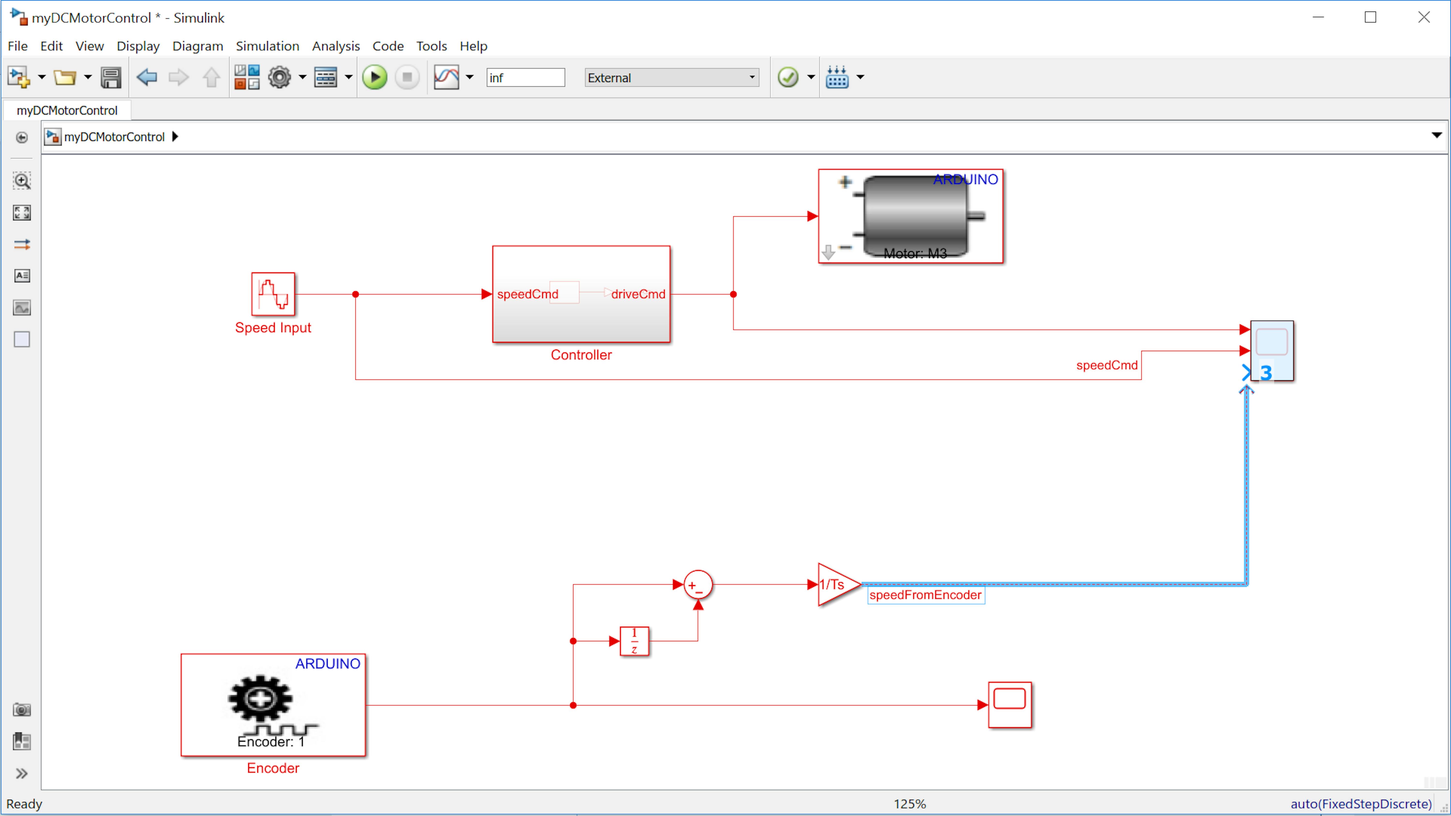
Make sure the MKR Motor Carrier power is ON and run the application on the MKR1000 board. Examine the Scope:
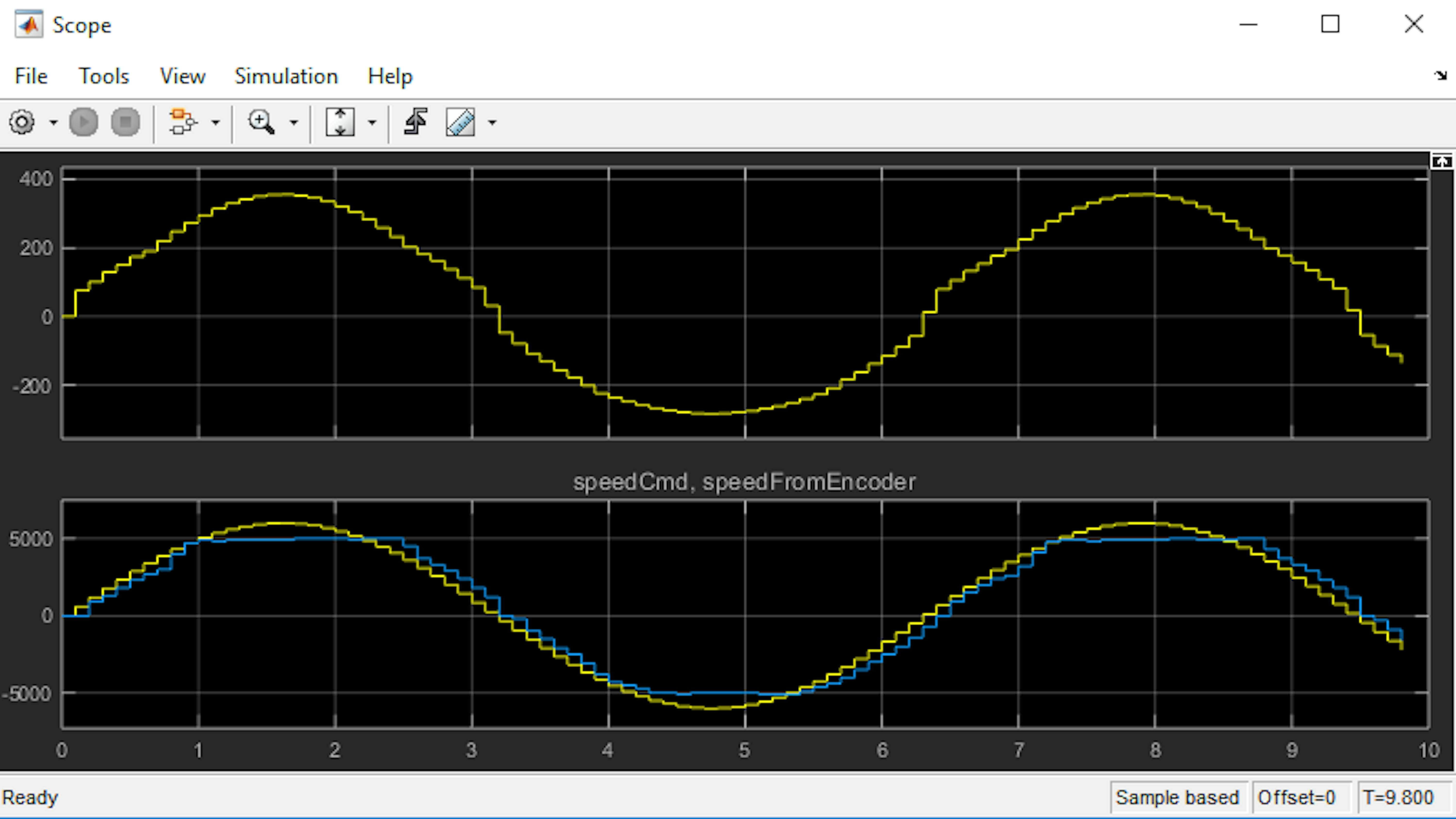
How does the measured speed compare to the commanded speed? Try slowing down the spinning motor with your finger.
How does the controller algorithm perform when an external torque load is applied? Stop the model.
To measure the performance of the controller, you need to see the error: the difference between the desired value and the actual (or measured) value of a quantity. To get the motor speed error, add a Sum block from Simulink > Math Operations with a List of Signs '|+-'. Branch and route the signals so that you are subtracting the speedFromEncoder signal from the speedCmd signal as shown below:

Drag the output signal from the Sum block to the Scope block, creating a new import in position 2 as shown here:
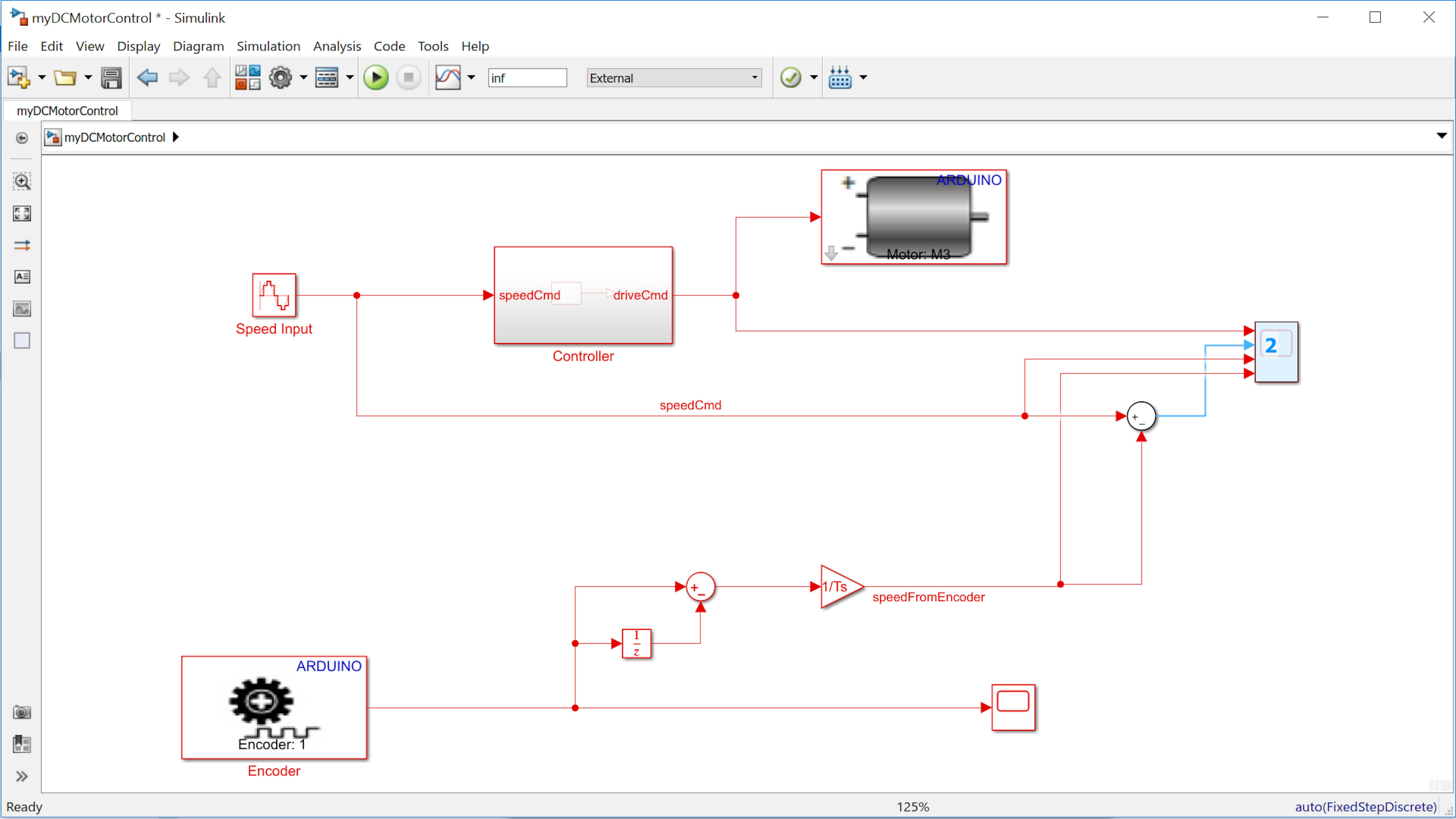
Label the new signal Error. Now go into the Scope block, and click View > Layout, and set the axes dimensions to 3x1:
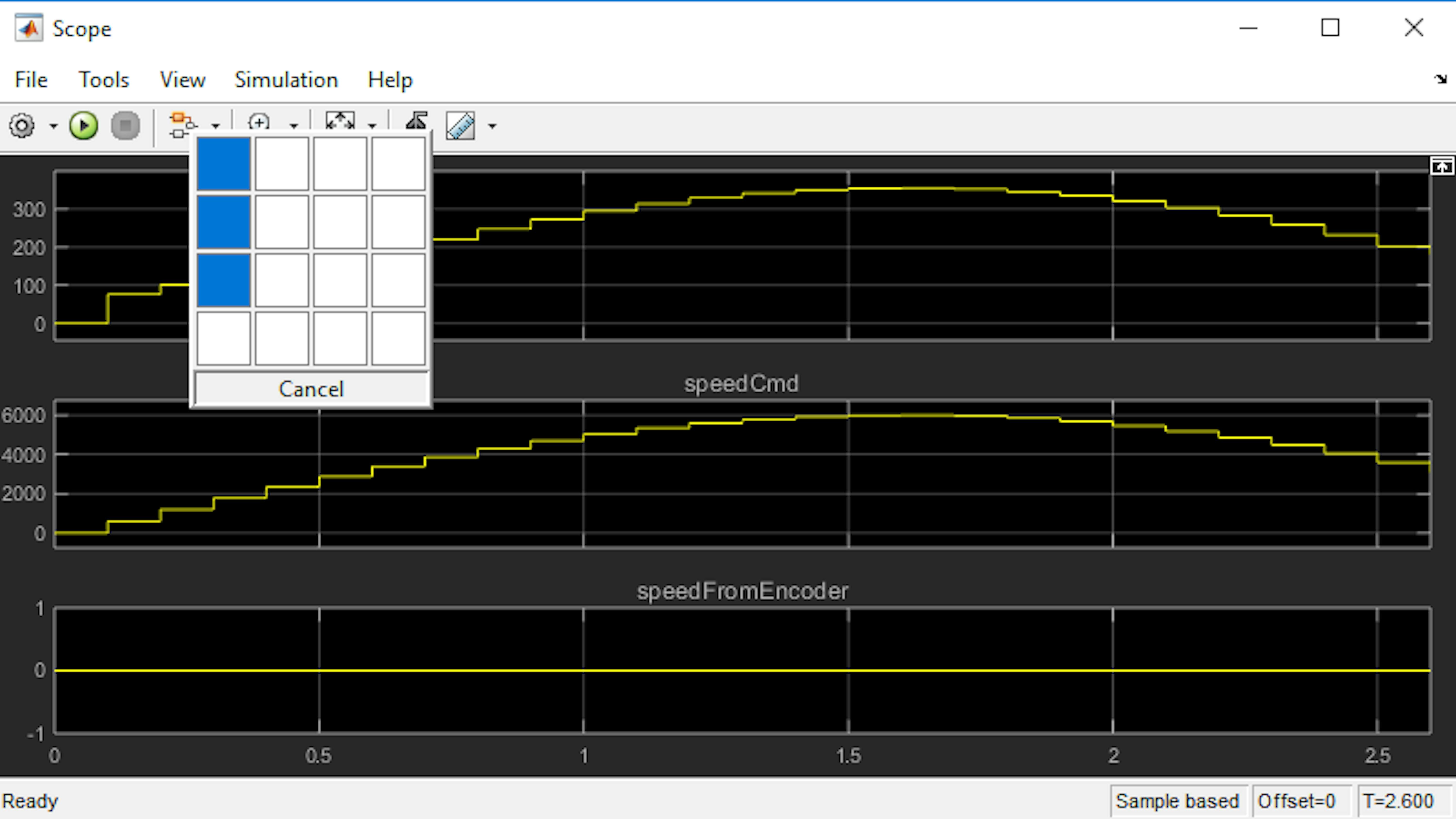
Run the model, and examine the signals in the Scope window:
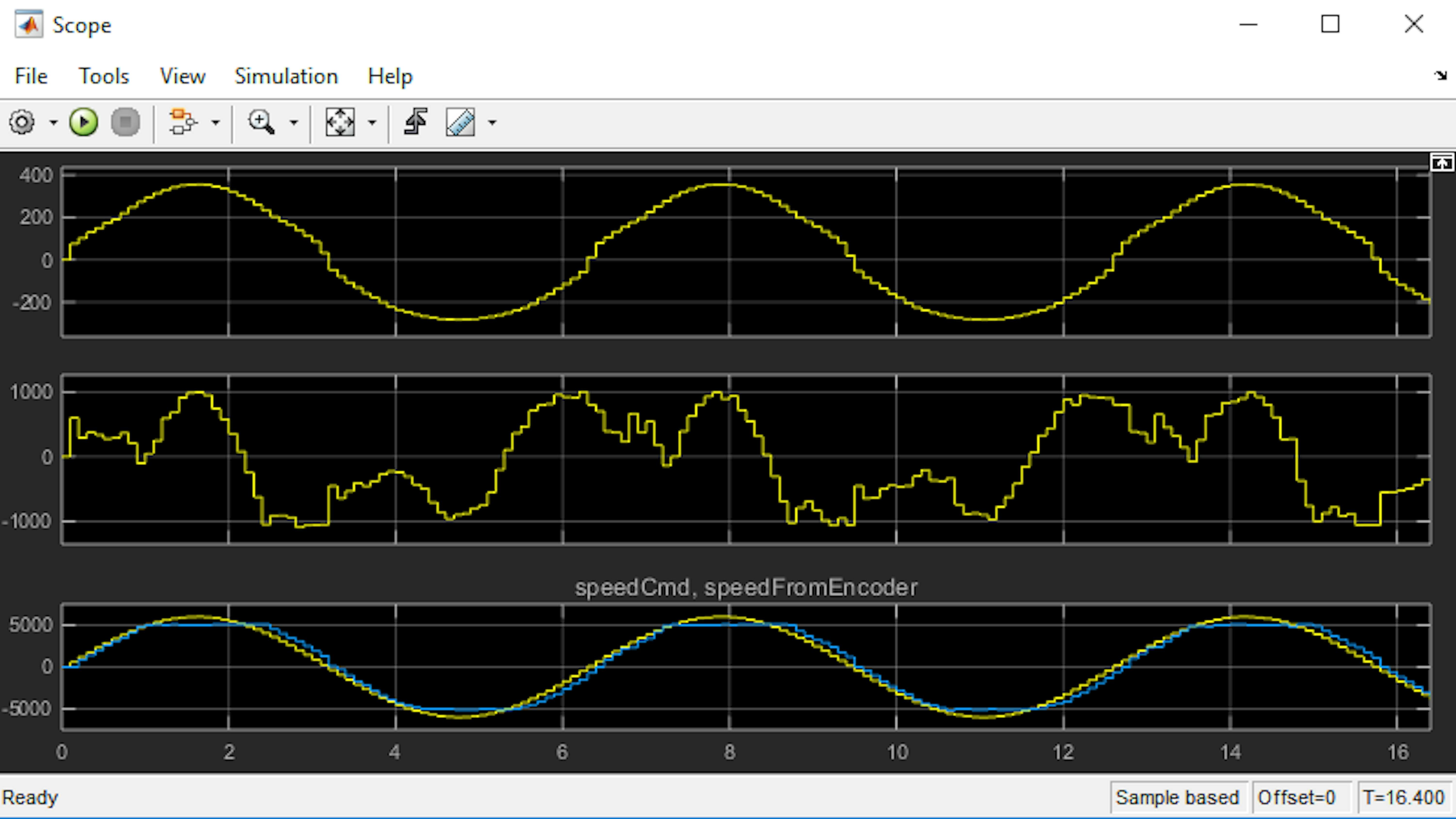
What you just implemented is open-loop control. In open-loop motor control, you have an algorithm that determines what drive command to send to the motor, and that drive command does not depend on the current state of the system. In other words, you are not considering the actual speed of the motor when determining the drive command. Open-loop control is useful when you have a very accurate model of your operating environment. In this case, the operating conditions are encompassed in the Lookup Table block. However, if there is any unmodeled torque acting on the motor, or you add a load (such as a wheel or gear), or the battery is not operating at the same voltage as when you generated the test data, open-loop control will not be sufficient.
How can you improve the accuracy of the motor control system? This is the question that we will address in the following section, where we will implement a closed-loop controller.
CLOSED-LOOP MOTOR CONTROL
To improve the performance of the controller when the operating conditions stray from the experimental conditions, you need to take the speed measurement into consideration when calculating the motor drive command.
Let's "close" the control loop by routing the speedFromEncoder measurement into the Controller subsystem. Branch off the speedFromEncoder signal and pass it into the Controller subsystem, creating a second inport:
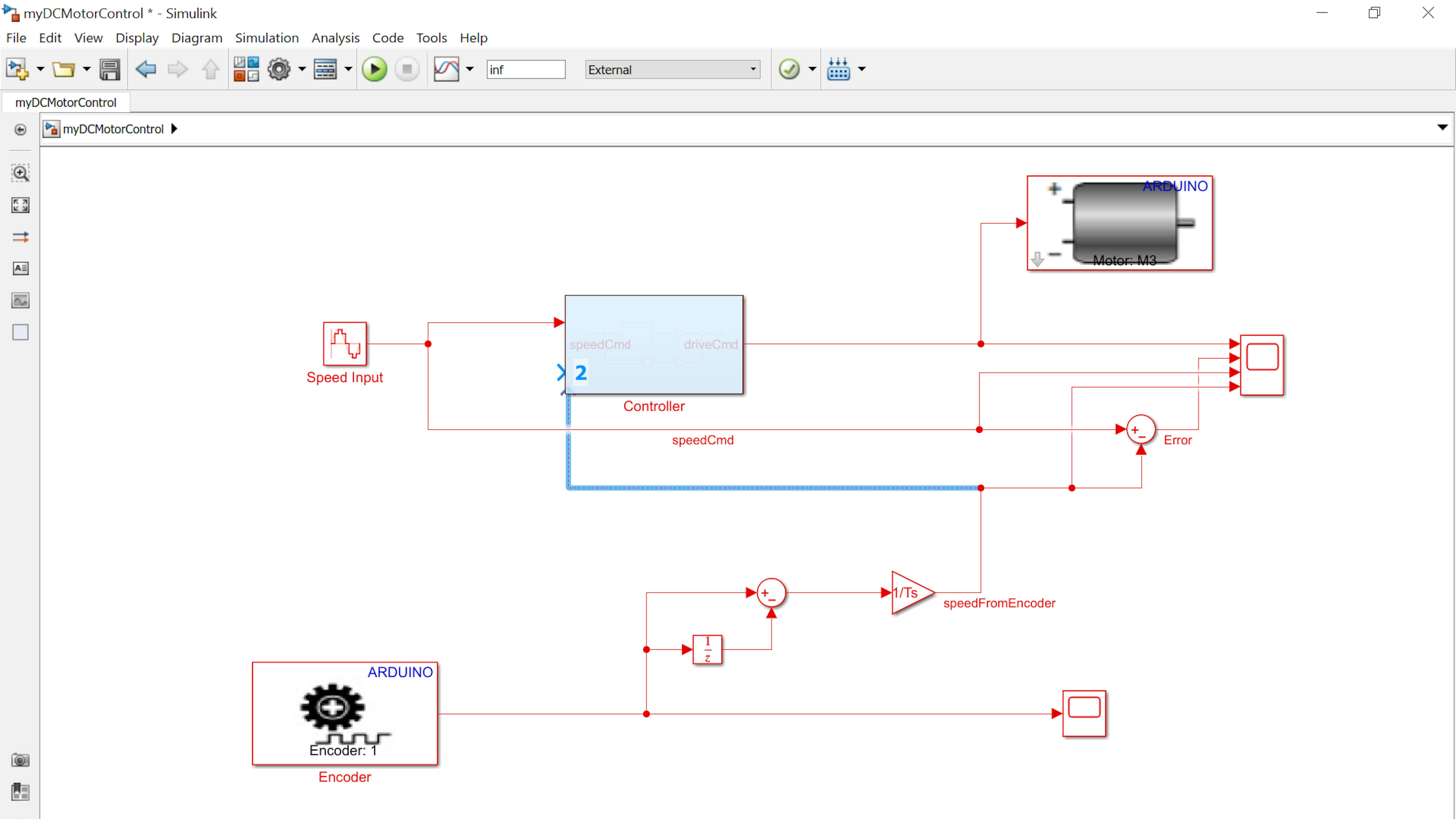
Next, let's access the speed error. Go inside the Controller subsystem, and add a Subtract block (from Simulink > Math Operations), then route the signals as shown below:

We are going to add a corrective term to the drive command that is proportional to the speed error. Add a Gain block to the Controller subsystem, and set the gain value to 0.01 (you will adjust this value later):
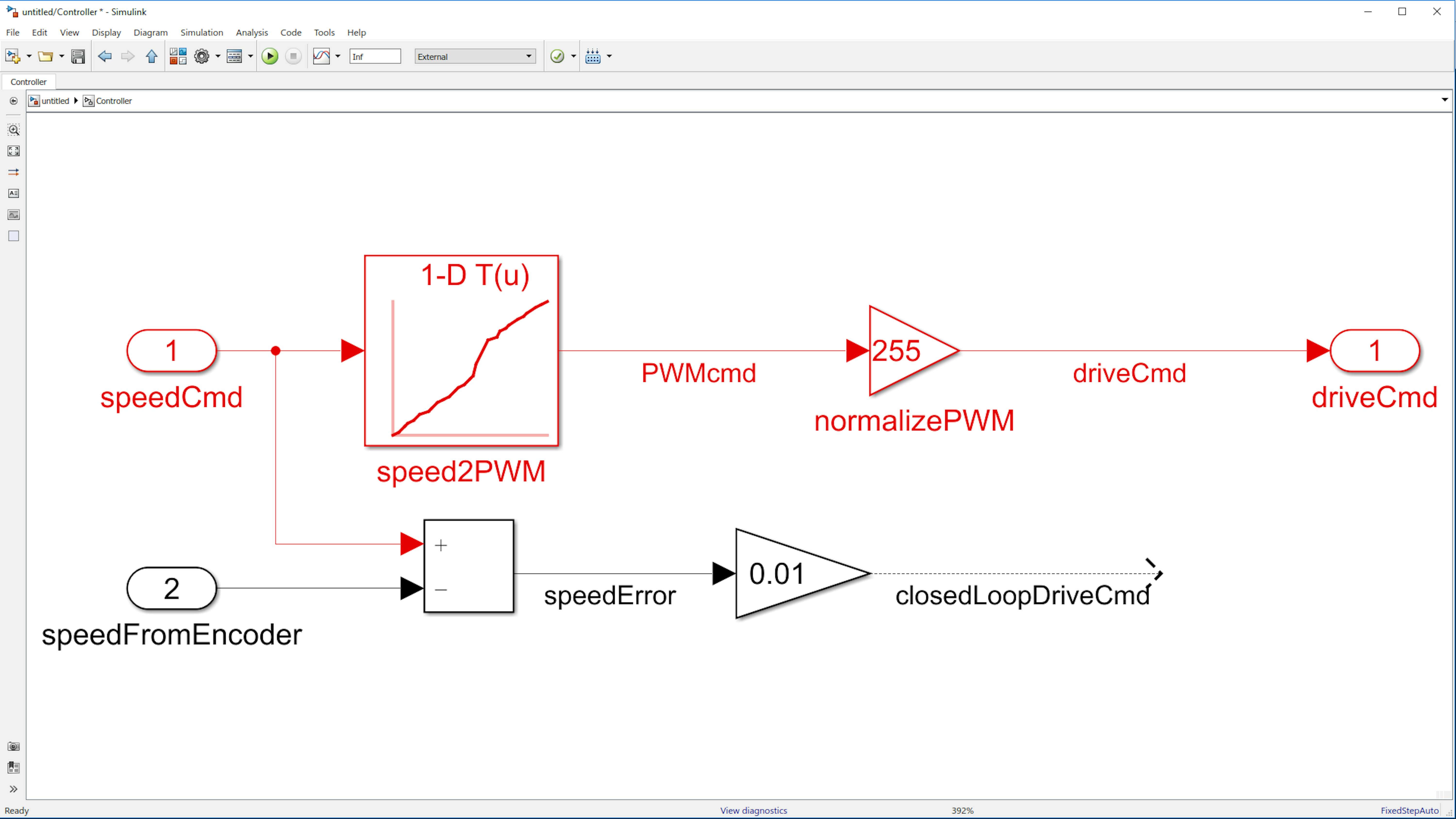
Now let's form the final drive command. Delete the driveCmd signal:
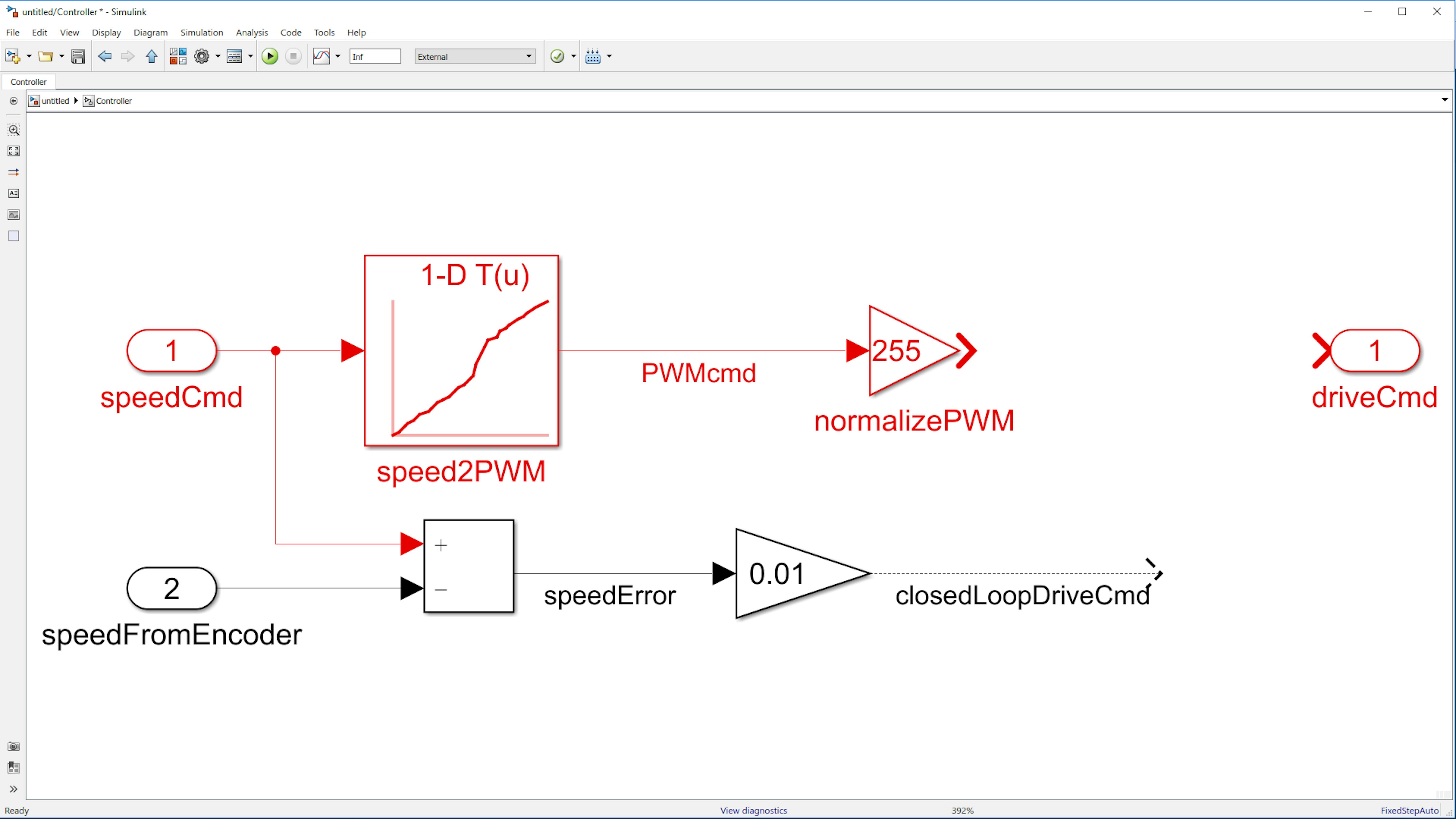
Now add a Sum block and route and label the signals as shown in the image below:
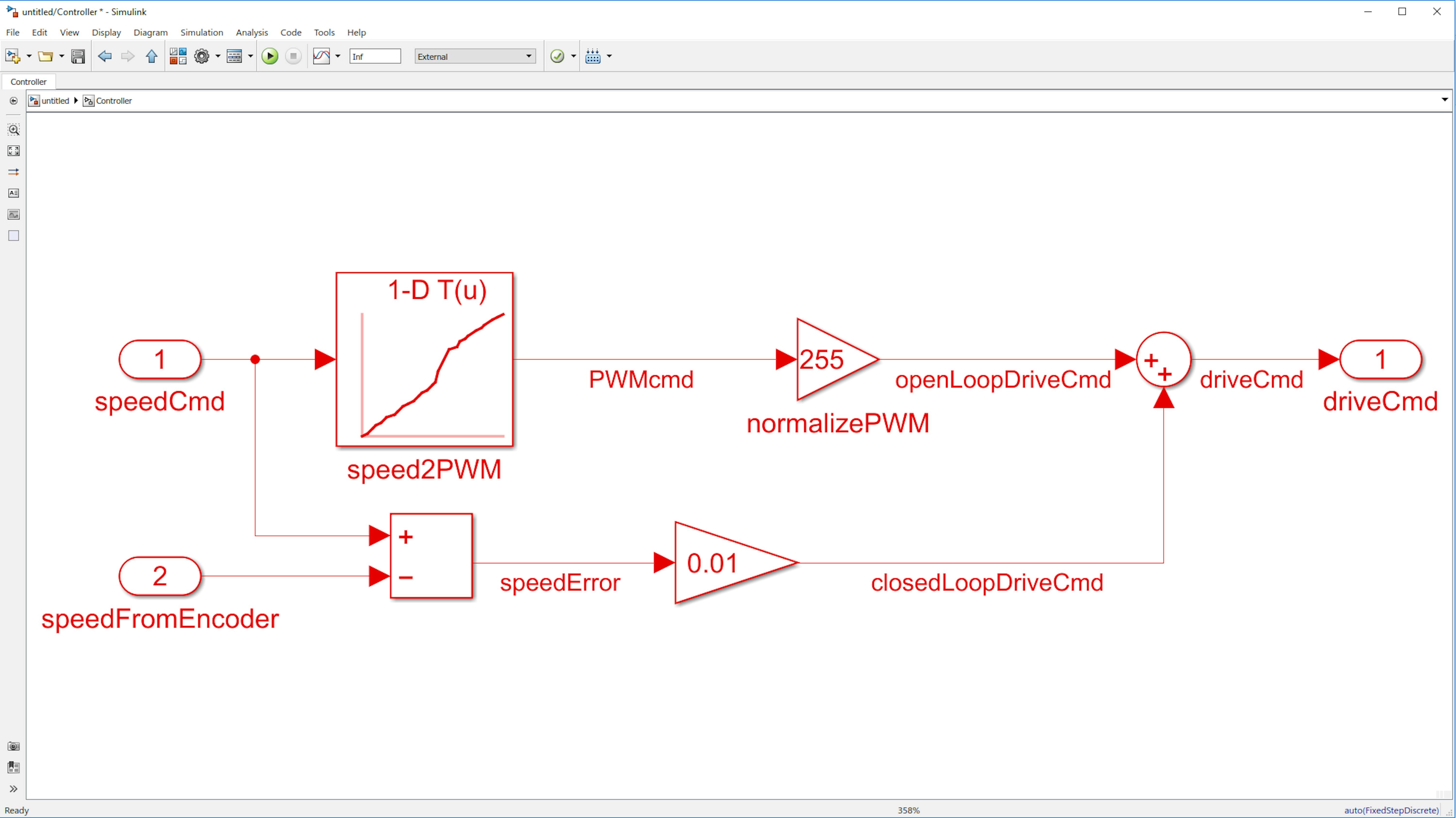
Let's try it out! Run the model on the MKR1000 board, and then examine the scope:
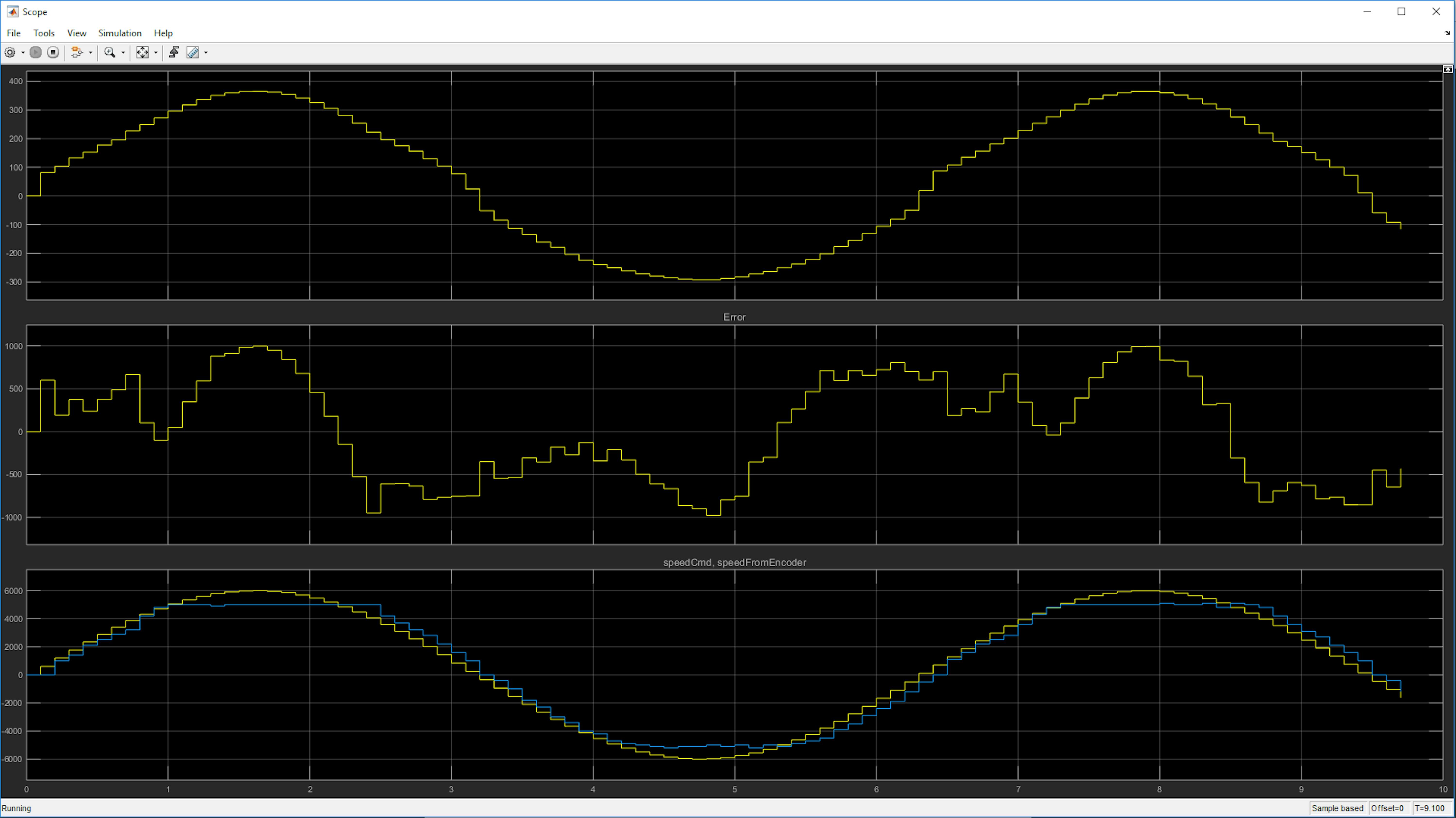
How does the performance compare to before?
While the application is running on the hardware, go back to the Gain block inside the Controller subsystem. Try different values of the gain. Click Apply to update the gain value on Arduino:
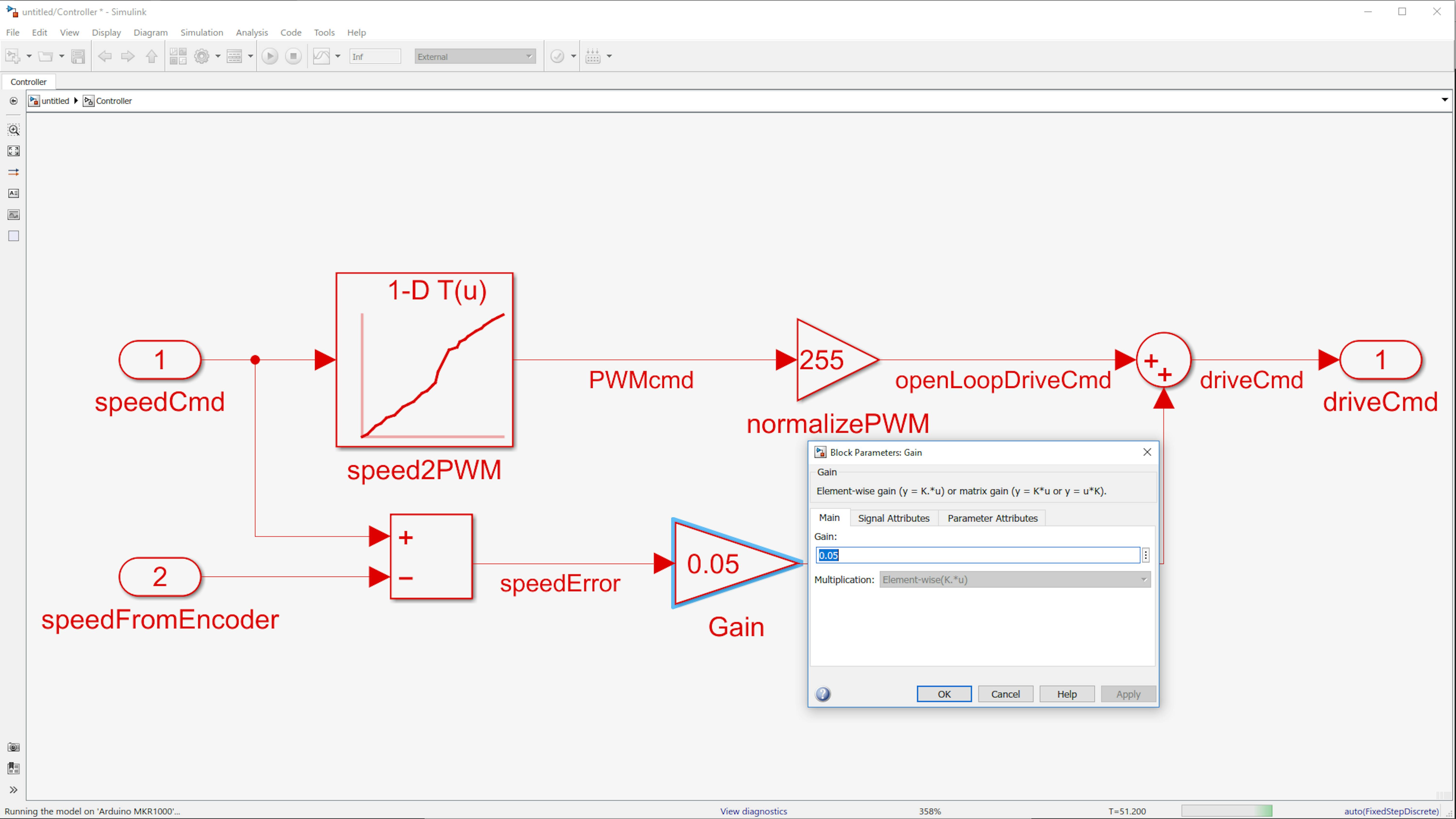
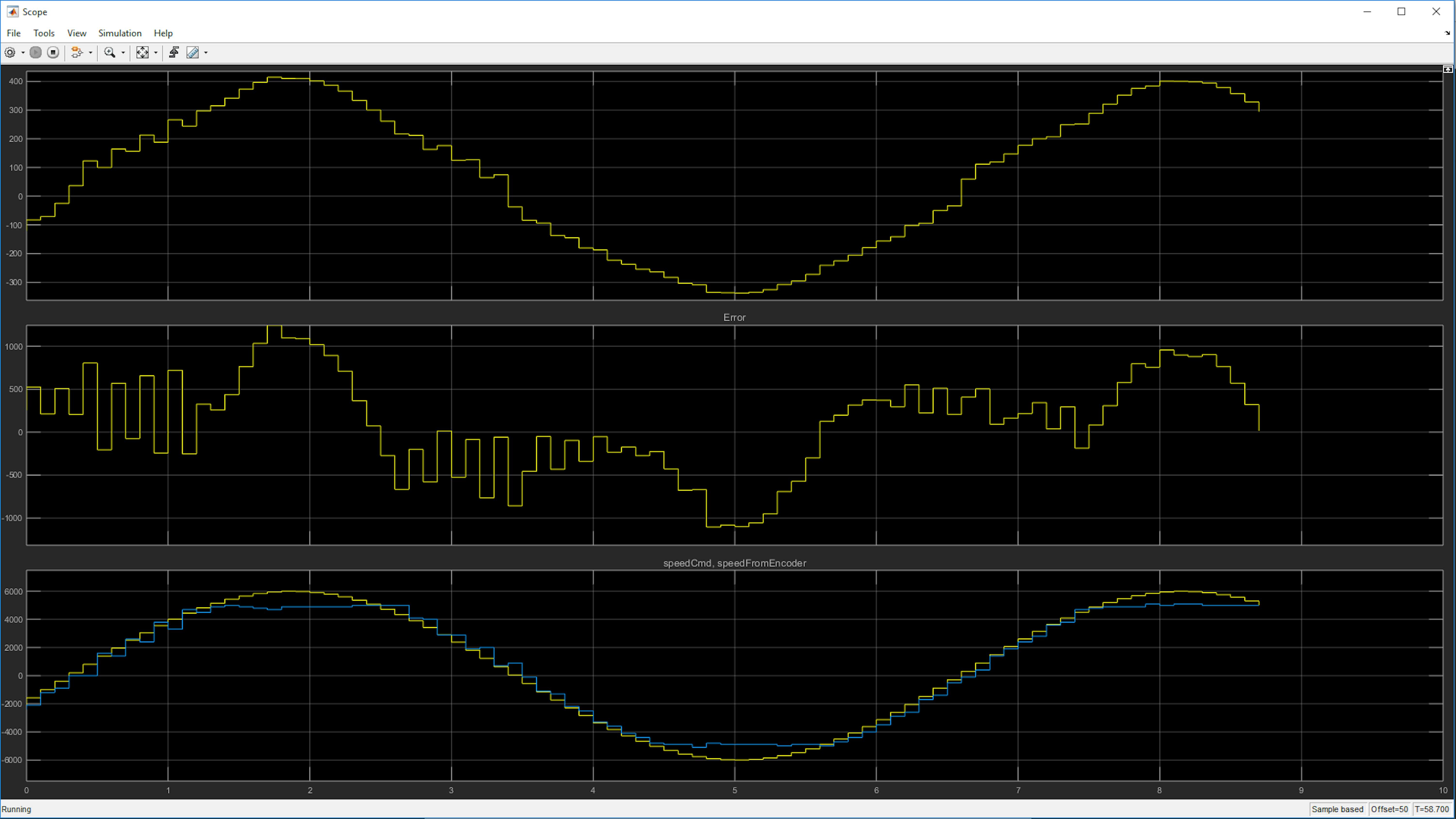
What gain value gives the best accuracy, higher or lower?
Continue running the application on Arduino. Now go into the Sine Wave block and change the waveform parameters. Try to answer the question: How robust is your controller at higher sine wave frequencies?
What you are doing now is called parameter tuning. By adjusting parameter values in the model as the application runs on the target hardware, you can gain valuable insight about how your system behaves under various circumstances and how best to parameterize the algorithm for the most robust performance.
DEPLOYING SIMULINK MODELS ON ARDUINO
Once you are satisfied with how your application performs in external mode, you will ultimately deploy your model as a standalone application, which can run without connecting to your computer. To build a standalone application, click the Deploy to Hardware button in the model window toolstrip:
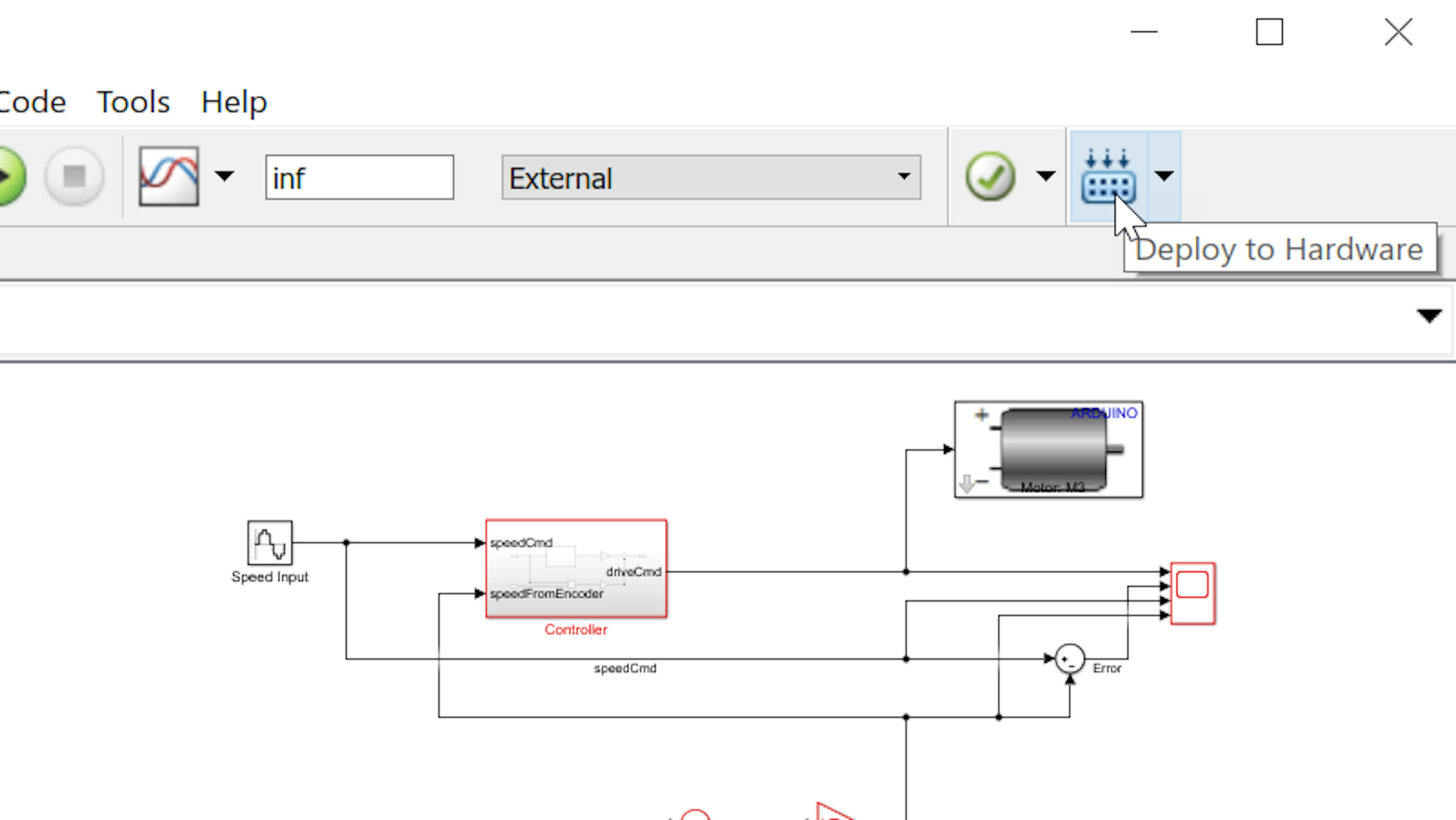
Once the build process completes, the application will immediately start running on Arduino. Notice that this time, the simulation is not running in the model window. You can now disconnect the USB cable between the MKR1000 board and your computer. The application continues to run. Now reconnect the USB cable to continue working.
You might have noticed that running an application in standalone mode relieves the processor of the performance overhead associated with external mode, producing better performance.